library(data.table)
library(flextable)
library(haven)
library(mirt)

anatomy_scale <-
  read_sav("data_folder.sav") |>
  as.data.table()

scale_items <-
anatomy_scale[, .SD, .SDcols = patterns("^Item")]Overview
This post walks through the application of confirmatory MIRT (Multidimensional Item Response Theory) models using data sourced from Kaşali et al. (2026), which outlines the adaptation and validation of an anatomy attitude scale for dental students. The scale consists of 14 items presented in the table below.
| Items | Factors |
|---|---|
| Item 1 | If I were the minister of health, I would abolish the anatomy course from dentistry faculties.* |
| Item 2 | Learning anatomy makes me happy. |
| Item 3 | I would not call a person who does not know anatomy a dentist. |
| Item 4 | If the most unnecessary courses are ranked, “anatomy” comes first.* |
| Item 5 | Anatomy information should be reminded at the beginning of each internship. |
| Item 6 | Recognising the human body with “anatomy” makes me feel like a dentist. |
| Item 7 | If I were in charge, I would remove anatomy information from the “Dentistry Speciality Examination”.* |
| Item 8 | If I were a dental education planner, I would recommend anatomy only as an elective course.* |
| Item 9 | I would like to do a PhD in anatomy when I graduate. |
| Item 10 | Drawing anatomical figures makes me happy. |
| Item 11 | I watch anatomy videos in my free time. |
| Item 12 | Anatomy practical lessons are interesting. |
| Item 13 | I liked anatomy very much because of the lecturers. |
| Item 14 | Anatomy is the basis of other dentistry courses. |
* Items written have negative meanings and scored reversely
The authors propose that Items 2, 3, 5, 6, 12, 13, and 14 load onto a valuing anatomy factor, Items 1, 4, 7, and 8 onto a hating anatomy factor, and Items 9, 10, and 11 onto an allocating-time-to-anatomy factor. Global fit for this three-factor structure was reported as acceptable: CFI = 0.922, TLI = 0.900.
Descriptive Statistics
Across the 14 items, descriptive statistics show reasonable variability in responses with no obvious endpoint piling. One data quality issue is worth flagging before proceeding: Item 4 contains a response value of 11, six points above the maximum scale value of 5. This is clearly an input error and has not been acknowledged or addressed in the published work. The value has been recoded to NA for all analyses here, as retaining it would affect item means and any downstream parameter estimates.
item_descriptives <-
  scale_items[, .(
    `Item ID` = as.integer(gsub("Item", "", names(.SD))),
    `Mean` = round(colMeans(.SD, na.rm = T), 2),
    `SD` = round(apply(.SD, 2, function (x) sd(x, na.rm = T)), 2),
    `Min` = apply(.SD, 2, function (x) min(x, na.rm = T)),
    `Max` = apply(.SD, 2, function (x) max(x, na.rm = T))
  )]

setorder(item_descriptives, `Item ID`)

item_descriptives |>
  flextable() |>
  align_nottext_col(align = "center")
Item ID | Mean | SD | Min | Max |
|---|---|---|---|---|
1 | 1.97 | 1.23 | 1 | 5 |
2 | 2.92 | 1.23 | 1 | 5 |
3 | 3.40 | 1.22 | 1 | 5 |
4 | 2.05 | 1.28 | 1 | 11 |
5 | 3.28 | 1.19 | 1 | 5 |
6 | 3.74 | 1.08 | 1 | 5 |
7 | 2.23 | 1.25 | 1 | 5 |
8 | 2.28 | 1.22 | 1 | 5 |
9 | 2.11 | 1.14 | 1 | 5 |
10 | 2.28 | 1.26 | 1 | 5 |
11 | 2.05 | 1.15 | 1 | 5 |
12 | 2.98 | 1.25 | 1 | 5 |
13 | 2.39 | 1.32 | 1 | 5 |
14 | 3.16 | 1.26 | 1 | 5 |
scale_items[, Item4 := fifelse(Item4 == 11, NA, Item4)]

scale_items[, .(
  `Item ID` = as.integer(gsub("Item", "", names(.SD))),
  `Mean` = round(colMeans(.SD, na.rm = T), 2),
  `SD` = round(apply(.SD, 2, function (x) sd(x, na.rm = T)), 2),
  `Min` = apply(.SD, 2, function (x) min(x, na.rm = T)),
  `Max` = apply(.SD, 2, function (x) max(x, na.rm = T))
), .SDcols = "Item4"] |>
  flextable() |>
  align_nottext_col(align = "center")
Item ID | Mean | SD | Min | Max |
|---|---|---|---|---|
4 | 2.02 | 1.17 | 1 | 5 |
neg_wrd <- c("Item1", "Item4", "Item7", "Item8")

scale_items[, (neg_wrd) := lapply(.SD, function (x) 6 - x), .SDcols = neg_wrd]
poly_mat <-
psych::polychoric(scale_items)$rho
corrplot::corrplot(poly_mat, type = "lower")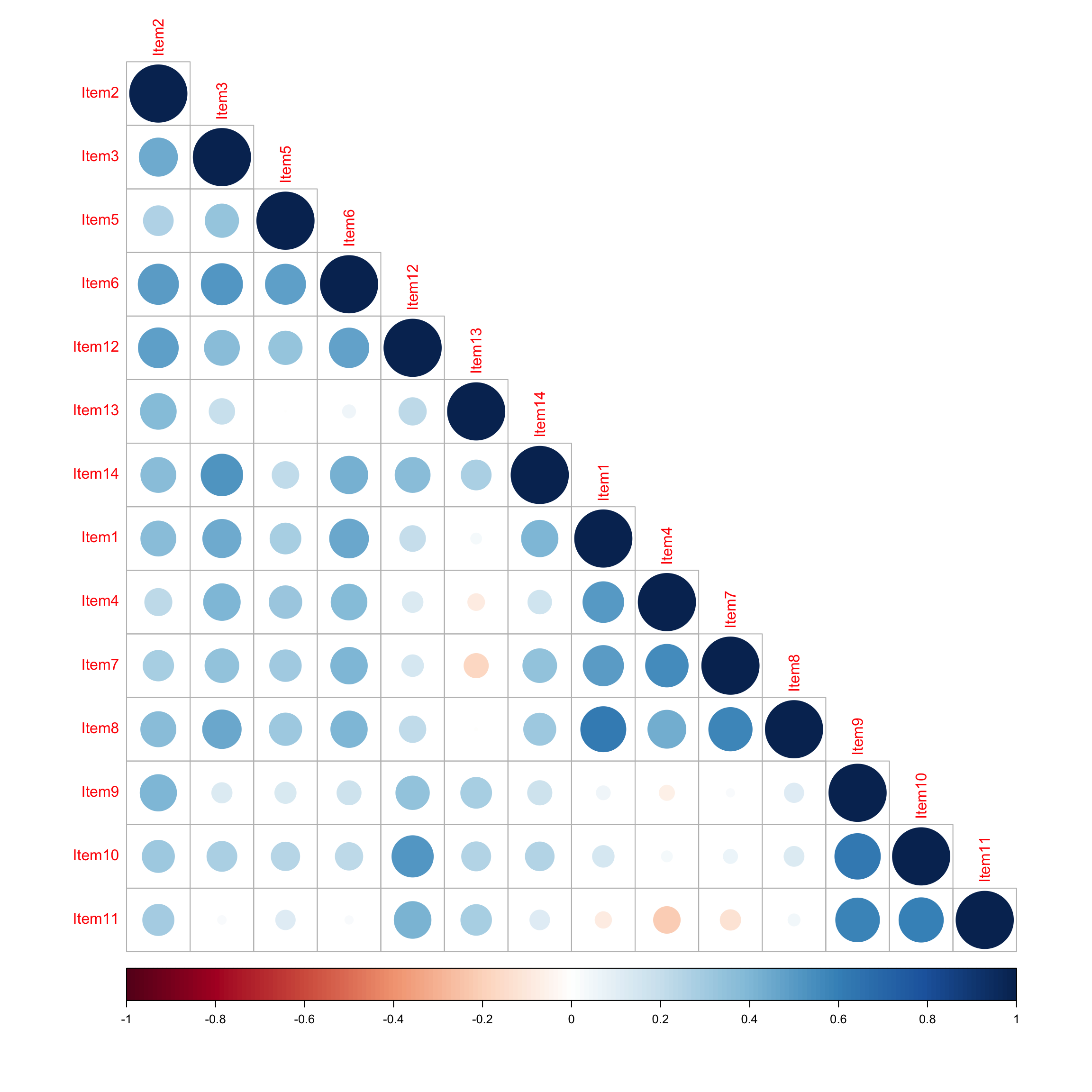
The correlation matrix shows several notable patterns. Item 13 is weakly correlated with most attitudinal items, with only modest correlations with the devoting-time-to-anatomy items. The item is written in the past tense and attributes positive sentiment toward anatomy to the quality of lecturers. This is a course satisfaction item, not an attitude toward anatomy as a discipline. It is theoretically orthogonal to intrinsic valuation of the subject, which is presumably what Factor 1 is meant to capture, and the correlation matrix makes this visible. Similar remarks apply to Item 12, which again asks about interest in a course rather than attitude toward anatomy itself. Both items reflect a content validity problem.
Items 9, 10, and 11 correlate strongly with each other. These are the items asking about anatomy engagement outside of formal coursework: watching videos, drawing figures, pursuing a research career. They show moderate correlations with Items 2, 12, and 13, which makes some sense: a student who appraises the course positively is more likely to engage with the subject in their own time, particularly if they are considering it as a career path.
Items 1, 4, 7, and 8 cluster as the “hating anatomy” factor, showing negative correlations with the positive attitude items (2, 3, 5, 6, 14). This pattern of positive and negative items splitting into separate factors is a well-documented wording artefact in attitude scale CFA. From the paper itself, the authors report a -0.67 correlation between the positive and negative attitudinal factors. What is likely happening is a methods effect is creating the perception of two distinct constructs, but the reality is a single bipolar attitude dimension. In other words, extracting a separate “Hating Anatomy” factor likely reflects the influence of item wording direction rather than anything substantive.
It’s also worth noting that devoting-time-to-anatomy items show near-zero or weakly negative correlations with the “hating anatomy” items. Someone who resents anatomy as a course requirement is not necessarily disinclined to watch anatomy videos. It appears that the two things are largely independent.
Aim
The approach taken is incremental, moving from a unidimensional through to a three-factor representation of the scale. Each model is evaluated on global and local fit, with preference placed on parsimony over factor overextraction.
Unidimensional Model
unidim_mod <-
  mirt(scale_items, model = 1, itemtype = "graded")
unidim_fit <- M2(unidim_mod)A single-factor graded response model converged after 29 iterations and demonstrated acceptable model fit, M2(35) = 67.94, p < 0.001, CFI = 0.93, TLI = 0.9, RMSEA = 0.06, 90% CI [0.04, 0.08].
The trace plots reveal two distinct problems. First, Items 11 and 13 show flattened category response curves, consistent with their low discrimination values in the item parameter table, both fall well below conventional cut-offs (a = 0.356 and a = 0.346 respectively). For both items, agreement categories occur only at extreme theta values, meaning they provide almost no information across the range of the latent trait where most respondents sit. Second, for several items the trace plots show clear peaks only for Strongly Disagree, Slightly Agree, and Strongly Agree; intermediate Disagree and Agree categories are relatively flat. This suggests the five-point response scale is functioning as three effective categories for much of the scale, which is a scale construction problem independent of the factor structure.
plot(unidim_mod, type = "trace")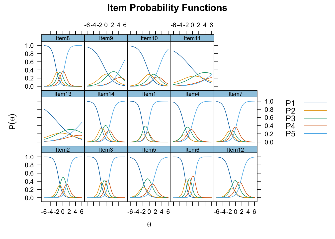
The item parameter table makes the issue with Items 9, 11, and 13 concrete. All three show severely disordered thresholds: for Item 13, b2 = 0.680 jumps to b3 = 4.350 and b4 = 6.25. These are threshold locations that fall far outside the range of any plausible respondent population. The Agree and Strongly Agree options are operationally inaccessible. Items 9 and 11 show the same pattern with b3 and b4 values of 3.587/4.969 and 5.995/8.545 respectively. These items are not functioning as five-point scales in any meaningful sense; for most respondents they are binary.
The remaining items show broadly ordered thresholds and reasonable discrimination values, with Items 3 and 6 performing best (a = 1.846 and a = 2.010). This pattern is consistent with the correlation matrix: Items 9, 11, and 13 are the weakest contributors to the unidimensional factor, and Item 13’s low loading adds further weight to the earlier argument that it is measuring course satisfaction rather than attitude toward anatomy as a discipline.
as.data.table(coef(unidim_mod, IRTpars = T, simplify = T)$items, keep.rownames = "Item ID") |>
  _[, `Item ID` := gsub("(?<=[A-Za-z])(?=\\d)", " ", `Item ID`, perl = T)] |>
  flextable() |>
  colformat_double(digits = 3) |>
  align_nottext_col(align = "center")
Item ID | a | b1 | b2 | b3 | b4 |
|---|---|---|---|---|---|
Item 2 | 1.591 | -1.397 | -0.608 | 0.767 | 1.636 |
Item 3 | 1.846 | -1.857 | -1.010 | -0.012 | 0.994 |
Item 5 | 1.121 | -2.349 | -1.416 | 0.375 | 1.605 |
Item 6 | 2.010 | -2.360 | -1.429 | -0.433 | 0.752 |
Item 12 | 1.230 | -1.608 | -0.827 | 0.626 | 1.941 |
Item 13 | 0.346 | -1.860 | 0.680 | 4.350 | 6.252 |
Item 14 | 1.308 | -1.914 | -0.814 | 0.500 | 1.413 |
Item 1 | 1.629 | -2.209 | -1.716 | -0.706 | -0.135 |
Item 4 | 1.152 | -2.856 | -2.242 | -0.924 | 0.177 |
Item 7 | 1.286 | -2.379 | -1.536 | -0.663 | 0.527 |
Item 8 | 1.528 | -2.304 | -1.370 | -0.423 | 0.575 |
Item 9 | 0.623 | -0.804 | 1.169 | 3.587 | 4.969 |
Item 10 | 0.816 | -0.829 | 0.639 | 2.122 | 3.259 |
Item 11 | 0.356 | -0.809 | 2.036 | 5.995 | 8.545 |
Two-Factor Model
# Columns are ordered by factors in the data, hence the discrepancy with item names
twf_syntax <- mirt.model(
  "
    ATT = 1-11
    DEV = 12-14

    COV = ATT*DEV
  "
)

twf_mod <-
  mirt(
    scale_items,
    model = twf_syntax,
    itemtype = "graded"
  )
twf_fit <- M2(twf_mod)A two-factor graded response model converged after 58 iterations and demonstrated global model fit comparable to, but not better than, the unidimensional model, M2(34) = 70.08, p < 0.001, CFI = 0.92, TLI = 0.89, RMSEA = 0.06, 90% CI [0.04, 0.08].
The discrimination improvements for Items 9, 10, and 11 on the DEV factor (a = 2.30, 2.63, and 1.91 respectively) are a meaningful result – under the unidimensional model these were among the weakest items, and freeing them onto a dedicated factor recovers substantial discriminating power. The two-factor solution is also competitive with the unidimensional model on global fit. However, collapsing value-of-anatomy and hating-anatomy into a single ATT factor leaves the internal structure of that factor unexamined, and the residual correlations suggest strain that a two-factor solution cannot resolve.
Item 13 remains problematic with a 0.282 discrimination value, and threshold disorder (b3 = 5.30 and b4 = 7.62). The remaining ten attitudinal items show no overt issues for either discrimination or threshold values.
as.data.table(coef(twf_mod, IRTpars = T, simplify = T)$items, keep.rownames = "Item ID") |>
  _[, `Item ID` := gsub("(?<=[A-Za-z])(?=\\d)", " ", `Item ID`, perl = T)] |>
  flextable() |>
  colformat_double(digits = 3) |>
  align_nottext_col(align = "center")
Item ID | a1 | a2 | b1 | b2 | b3 | b4 |
|---|---|---|---|---|---|---|
Item 2 | 1.486 | 0.000 | -1.454 | -0.630 | 0.802 | 1.702 |
Item 3 | 1.837 | 0.000 | -1.866 | -1.021 | -0.017 | 1.002 |
Item 5 | 1.113 | 0.000 | -2.366 | -1.430 | 0.377 | 1.615 |
Item 6 | 2.017 | 0.000 | -2.359 | -1.433 | -0.434 | 0.759 |
Item 12 | 1.112 | 0.000 | -1.725 | -0.887 | 0.671 | 2.076 |
Item 13 | 0.282 | 0.000 | -2.266 | 0.825 | 5.300 | 7.623 |
Item 14 | 1.289 | 0.000 | -1.933 | -0.828 | 0.503 | 1.431 |
Item 1 | 1.731 | 0.000 | -2.139 | -1.665 | -0.689 | -0.131 |
Item 4 | 1.260 | 0.000 | -2.682 | -2.111 | -0.874 | 0.169 |
Item 7 | 1.404 | 0.000 | -2.248 | -1.458 | -0.634 | 0.502 |
Item 8 | 1.624 | 0.000 | -2.227 | -1.335 | -0.414 | 0.563 |
Item 9 | 0.000 | 2.302 | -0.359 | 0.480 | 1.522 | 2.122 |
Item 10 | 0.000 | 2.627 | -0.428 | 0.361 | 1.126 | 1.689 |
Item 11 | 0.000 | 1.909 | -0.212 | 0.581 | 1.635 | 2.310 |
Residual correlations flag localised strain between Item 13 and Item 2, and between Items 1, 4, 7, 8 and the positive attitudinal items. The Item 2/13 strain indicates these items correlate more strongly than the factor structure accounts for, and is interpretable given that both touch on positive affect toward anatomy, but for different reasons: Item 2 captures intrinsic enjoyment of learning the subject, while Item 13 attributes positive valuation externally to teaching staff. The residual strain between the negatively-worded items (1, 4, 7, 8) and the positive attitudinal cluster reflects the bipolar attitude dimension discussed earlier. Someone who intrinsically values anatomy is unlikely to endorse calls for its removal from the curriculum.
twf_resid <- residuals(twf_mod, "Q3")corrplot::corrplot(twf_resid, method = "number", type = "lower")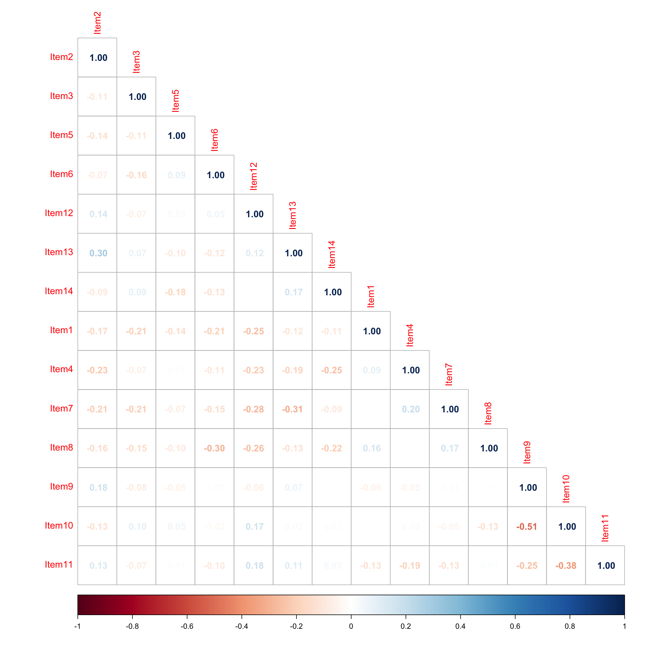
Three-Factor Model
thf_syntax <- mirt.model(
  "
    VAL = 1-7
    HAT = 8-11
    DEV = 12-14

    COV = VAL*HAT*DEV
  "
)

thf_mod <-
  mirt(
    scale_items,
    model = thf_syntax,
    itemtype = "graded"
  )
thf_fit <- M2(thf_mod)A three-factor graded response model converged after 30 iterations and still demonstrated worse model fit than the unidimensional model, M2(32) = 91.04, p < 0.001, CFI = 0.87, TLI = 0.81, RMSEA = 0.08, 90% CI [0.06, 0.1]. The fit trajectory across models is worth stating plainly: the unidimensional model (CFI = 0.93) and two-factor model (CFI = 0.92) perform comparably, while the three-factor solution (CFI = 0.87) is the worst of the three. On parsimony grounds, neither multifactor solution earns its additional complexity.
The discrimination values for the negatively-worded items improve substantially once they load onto a dedicated HAT factor. Items 1, 4, 7, and 8 reach a = 2.268, 1.731, 2.008, and 2.297 respectively. These items are suppressed when collapsed with the positive attitudinal items and perform well when separated. Still the likelihood is that this is not a distinct factor that sits separately – the interfactor correlation between VAL and HAT of r = 0.68 adds further weight to this point.
Item 13 shows modest improvements in this model. The discrimination rises to a = 0.487 and the upper thresholds reduce to b3 = 3.171 and b4 = 4.540. A discrimination value below 0.50 remains well below any conventional threshold for a useful item, and threshold locations of 3.17 and 4.54 still place the upper response categories beyond the range of any plausible respondent. Item 13 is less problematic in this model than in the previous two, but is not functioning adequately in any of them.
The DEV factor (Items 9, 10, 11) continues to perform well, with discrimination values of a = 2.318, 2.687, and 1.966, which is consistent with this being a separate factor altogether. This is further substantiated with the low to moderate inter-factor correlations with VAL and HAT (0.488 and 0.102 respectively).
Taken together, the three-factor model confirms that the devoting-time items constitute a distinct factor, and that the value-versus-hating distinction is a tenuous claim.
as.data.table(coef(thf_mod, IRTpars = T, simplify = T)$items, keep.rownames = "Item ID") |>
  _[, `Item ID` := gsub("(?<=[A-Za-z])(?=\\d)", " ", `Item ID`, perl = T)] |>
  flextable() |>
  colformat_double(digits = 3) |>
  align_nottext_col(align = "center")
Item ID | a1 | a2 | a3 | b1 | b2 | b3 | b4 |
|---|---|---|---|---|---|---|---|
Item 2 | 1.763 | 0.000 | 0.000 | -1.297 | -0.556 | 0.738 | 1.558 |
Item 3 | 1.870 | 0.000 | 0.000 | -1.831 | -0.968 | 0.027 | 1.004 |
Item 5 | 1.137 | 0.000 | 0.000 | -2.310 | -1.377 | 0.394 | 1.601 |
Item 6 | 2.044 | 0.000 | 0.000 | -2.342 | -1.391 | -0.396 | 0.757 |
Item 12 | 1.502 | 0.000 | 0.000 | -1.393 | -0.701 | 0.578 | 1.727 |
Item 13 | 0.487 | 0.000 | 0.000 | -1.331 | 0.516 | 3.171 | 4.540 |
Item 14 | 1.417 | 0.000 | 0.000 | -1.799 | -0.744 | 0.496 | 1.352 |
Item 1 | 0.000 | 2.268 | 0.000 | -1.886 | -1.496 | -0.637 | -0.125 |
Item 4 | 0.000 | 1.731 | 0.000 | -2.206 | -1.757 | -0.748 | 0.136 |
Item 7 | 0.000 | 2.008 | 0.000 | -1.856 | -1.239 | -0.559 | 0.423 |
Item 8 | 0.000 | 2.297 | 0.000 | -1.874 | -1.180 | -0.382 | 0.496 |
Item 9 | 0.000 | 0.000 | 2.318 | -0.346 | 0.483 | 1.521 | 2.113 |
Item 10 | 0.000 | 0.000 | 2.687 | -0.415 | 0.359 | 1.121 | 1.678 |
Item 11 | 0.000 | 0.000 | 1.966 | -0.202 | 0.577 | 1.617 | 2.279 |
Final Model
Based on the above analyses, two decisions are made. Item 13 is dropped for having a consistently low discrimination value across all three models – it fails to function as an attitude item. Items 9, 10, and 11 are dropped – they capture self-reported behaviours and behavioural intentions rather than affective attitudes towards anatomy. They remain relevant in the wider attitudinal model, wherein intentions are assumed to be associated with both affective and cognitive factors. However, this model is designed to solely capture affective attitudes towards anatomy. As the authors note, the scale is intended to measure attitudes towards anatomy, not intentions to complete a PhD or watching videos.
scale_items[, c("Item13", "Item9", "Item10", "Item11") := NULL]

final_mod <-
  mirt(
    scale_items,
    model = 1,
    itemtype = "graded"
  )
final_fit <- M2(final_mod)The 10-item single factor graded response model converged after 33 iterations and demonstrated excellent model fit, M2(5) = 7.14, p = 0.21, CFI = 0.98, TLI = 0.94, RMSEA = 0.04, 90% CI [0, 0.1]. This is an improvement over both the original paper’s reported fit indices and any other solutions considered above.
Discrimination values for the 10-item model are good, ranging from 1.008 to 1.811, and thresholds appear ordered.
as.data.table(coef(final_mod, IRTpars = T, simplify = T)$items, keep.rownames = "Item ID") |>
  _[, `Item ID` := gsub("(?<=[A-Za-z])(?=\\d)", " ", `Item ID`, perl = T)] |>
  flextable() |>
  colformat_double(digits = 3) |>
  align_nottext_col(align = "center")
Item ID | a | b1 | b2 | b3 | b4 |
|---|---|---|---|---|---|
Item 2 | 1.371 | -1.526 | -0.659 | 0.844 | 1.785 |
Item 3 | 1.791 | -1.894 | -1.040 | -0.021 | 1.018 |
Item 5 | 1.098 | -2.395 | -1.450 | 0.379 | 1.632 |
Item 6 | 1.985 | -2.382 | -1.448 | -0.438 | 0.770 |
Item 12 | 1.008 | -1.855 | -0.952 | 0.721 | 2.225 |
Item 14 | 1.242 | -1.983 | -0.855 | 0.512 | 1.468 |
Item 1 | 1.811 | -2.093 | -1.632 | -0.677 | -0.127 |
Item 4 | 1.360 | -2.553 | -2.011 | -0.836 | 0.161 |
Item 7 | 1.520 | -2.145 | -1.397 | -0.611 | 0.481 |
Item 8 | 1.699 | -2.171 | -1.311 | -0.408 | 0.555 |
The trace plots show this not to be the case – majority of response scales could be collapsed into three-points. Response options 2 (Disagree) and 4 (Agree) never dominate at any theta level – their category response functions are overlapping. For majority of students completing this scale, these response options are avoided; the same finding was reported with the 14-item unidimensional model. Therefore, it is recommended to consider a three-point scale in future uses of this scale over the current five-point approach.
plot(final_mod, type = "trace")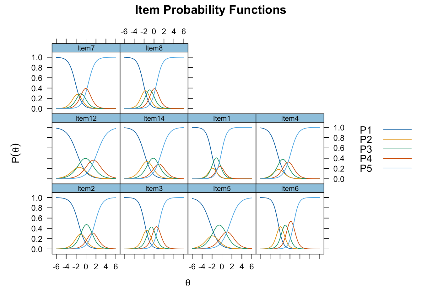
Finally, it is worth noting that this model collapses both positively and negatively worded items onto a single factor, contrary to the original authors’ findings. The negatively worded items appear to have produced a method effect in the original CFA that is not considered – the factor separation appears more consistent with a wording-related methods effect than with clearly distinct psychological constructs. It makes more sense to treat attitude toward something as bipolar, ranging from negative to positive. It would be difficult to conceive of an individual simultaneously holding strong negative attitudes (wanting to remove a course from the curriculum) and strong positive ones (finding learning anatomy genuinely enjoyable).
Summary
Through the application of confirmatory MIRT models, it has been shown that the original validation is not well supported. It is another instance of adapting a scale to a new cohort and assuming the underlying psychometric model transfers with it. The original paper’s global fit indices fell short of what is considered good, and the analysis here shows why: local fit problems, threshold disorder, and a factor structure driven by item wording direction rather than distinct attitude dimensions are all visible once the appropriate models are applied. Global fit alone is insufficient – it needs to be supplemented with local fit inspection and systematic comparison of competing model representations, rather than treating the original structure as the default.
The scale is workable, but not as published. Two coherent dimensions emerge from the data: affective attitude toward anatomy, and devoting-time-to-anatomy as a behavioural indicator. Splitting the attitudinal dimension into positive and negative valences is not supported – interfactor correlations are high and the unidimensional solution fits as well as or better than any multifactor alternative, with none of the added complexity. It is theoretically implausible that an individual would simultaneously hold strongly positive and strongly negative attitudes toward the same object.
Three recommendations follow. First, Item 13 should be dropped – it measures course satisfaction rather than attitude toward anatomy and does not function adequately under any model tested. Second, the five-point response scale should be collapsed to three points, reflecting how respondents are actually using it. Third, the behavioural items (9, 10, 11) should be treated as a separate measure, retained only where the devoting-time dimension is theoretically meaningful to the end user.