library(data.table)
library(ggplot2)
library(patchwork)
library(reticulate)
library(scales)Computerised Adaptive Tests (CAT) are assessments that adapt to an individual’s ability. It does this by adjusting the difficulty of the question you receive based on how you are answering. If you’re answering all questions correctly, then you’ll receive more difficult items. The more you get wrong, the easier items you’ll see. With each response given, the CAT re-estimates your ability. At the end of the assessment, a final ability is produced, upon which a decision is made. This could be whether you get to the next stage of in the job application process.

In this post, we’ll walk through how CATs work, but also how to simulate the completion of a CAT!
Setting Up a Simulation Study
To show the workings of a CAT, we’ll use the catsim Python package.
from catsim.cat import generate_item_bank
from catsim.estimation import NumericalSearchEstimator
from catsim.initialization import RandomInitializer
from catsim.selection import RandomesqueSelector
from catsim.simulation import Simulator
from catsim.stopping import MaxItemStopper
import numpy as np
Item Banks
Any CAT has an item bank. It contains all the possible items you could be shown during an assessment. The bank is large in size to reduce items becoming compromised due to over-exposure. If you only had 50 items and every candidate saw 25 items, it wouldn’t take many attempts for all items to be seen. This is also an issue given the numerous “Homework Helping” sites where answers can be found.
So, in an item bank, we’d have the index of each question, the question text, the possible answers, and answer key. In addition, you’ll find parameters associated with each item:
Item Discrimination: Shows how well the question discriminates between low and high ability candidates. A higher value means the question better differentiates abilities.
Item Difficulty: The ability value at which a candidate has a 50% likelihood of getting the question correct.
Pseudo-Guessing: The probability that, through guessing alone, you would answer the question correctly.
The parameters depend on the Item Response Theory model that is used. Here, we look at the 1 Parameter model. This is where only the item difficulty value can vary across questions. No guessing is accounted for and all items are assumed differentiate.
np.random.seed(20240314)

# Item Bank Generation
item_bank = generate_item_bank(
    n=400,
    itemtype="1PL"
)
Initial Ability
When you start an assessment, we don’t know your ability. Therefore, an initial ability estimate is used, which is sampled from a distribution. This initial ability determines the first question you get. In our case, we can sample from either the normal or uniform distribution. We use a uniform distribution here, which gives all values within a range (-3 to 3) an equal probability of being selected. If a normal distribution were selected, values towards the centre of the distribution would be more likely than those towards the distribution tails.
# Initial ability estimate for a test taker
initial_ability_estimate = RandomInitializer(
  dist_type="uniform",
  dist_params=(-3,3)  # Using a uniform distribution ranging from -3 to 3
)
Item Selection
We have our question and we have an initial ability, but no way to select a question. There are various techniques available. In this case, the Randomesque approach is used. It involves randomly selecting a question from a subset of the most informative items. In other words, given the ability estimate, what are the items closest in terms of difficulty. In our case, we are selecting the 5 closest items and then randomly selecting one.
# Selecting the next item for the test taker
random_item_selector = RandomesqueSelector(
    bin_size=5  # We select the 5 closest items in terms of difficulty to randomly sample from
)
Updating the Ability Estimate
The answer to each question is recorded. Based on the item parameters (e.g., item difficulty), the new ability estimate is based on the one that maximises the likelihood the individual’s pattern of correct/incorrect responses.
# Ability Estimator based on response correctness
ability_estimator = NumericalSearchEstimator()
Stopping the CAT
At some point, the CAT needs to stop. This could be through the number of questions completed or based on the variability in the ability estimate. It’s typically a balance. You want the best estimate of someone’s ability, but you don’t want someone completing a million questions. This is where simulations can help. You can use them to determine the optimal number of questions to present, whilst ensuring the best ability estimate is obtained. Here, we set the stopping criteria to a maximum of 25 items.
# Stopping Logic
max_item_stop = MaxItemStopper(
  max_itens=25  # Setting the stopping criteria to 25 items
  )
Running the Simulation
All the CAT components are set. We can now run the simulation and we can specify how many ‘examinees’ we want.
# Run CAT Simulation
cat_simulation = Simulator(
  items=item_bank,
  examinees=1000
)
cat_simulation.simulate(
  initializer=initial_ability_estimate,
  selector=random_item_selector,
  estimator=ability_estimator,
  stopper=max_item_stop,
)
Item Exposure Rates
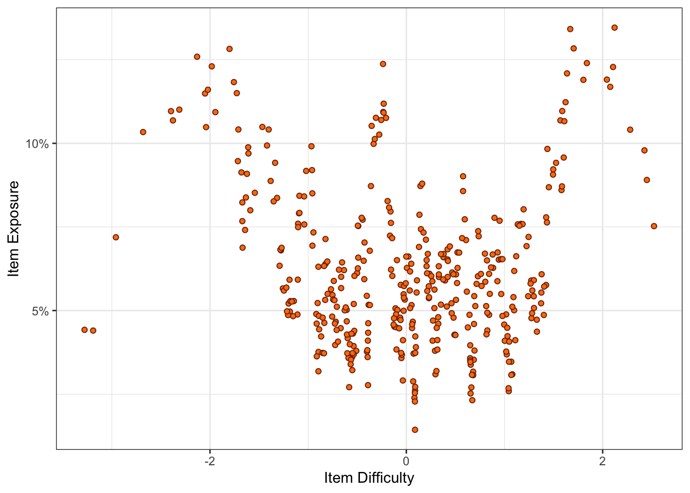
From our simulation, we can obtain various results. The first is the item exposure rate. One reason for running such simulations is to check how it would affect exposure of questions within the item bank. We could vary the item selection method and see the impact that has on exposure, for instance.
Figure 1 plots the item exposure rates by individual item difficulty values. It seems that easier (item difficulty values < -1) and harder (item difficulty values > 1) have the greatest exposure values. The reason is because the item difficulty values are based on a normal distribution (M=0, SD=1). The result is that there are few items with difficulty values at the extremes. So when we are selecting the next item using the Randomesque method, there are fewer candidate items to select from. Therefore, the few items at the extreme become overexposed.
py$cat_simulation$items |>
  as.data.table() |>
  ggplot(aes(x = V2, y = V5)) +
  geom_jitter(
    colour = "#78290f",
    fill = "#ff7d00",
    shape = 21
  ) +
  theme_bw() +
  labs(
    x = "Item Difficulty",
    y = "Item Exposure"
  ) +
  scale_y_continuous(
    labels = percent_format()
  )
Ability Estimate
From the simulation results, you can obtain the various information for each examinee:
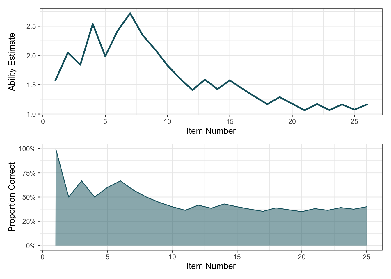
Ability Estimates: For each examinee, we can obtain a list of their ability estimates between the start and end points of the assessment. It shows how ability estimates of an examinee change given the correctness of a response to a question.
Response Vectors: This is a list of whether the examinee’s response to each question was correct or incorrect.
Administered Items: Based on the ability estimate, what items did the examinee see during the assessment.
ability_estimates = cat_simulation.estimations[0]  # Ability estimates for examinee 1
response_vector = cat_simulation.response_vectors[0]  # Response vector for examinee 1
administered_items = cat_simulation.administered_items[0]  # Questions examinee 1 saw
administered_item_details = cat_simulation.items[administered_items]  # Details for the administered questions that examinee 1 saw
ability_estimates <-
py$ability_estimates |>
as.double() # Convert from list to vector
administered_item_details <-
py$administered_item_details # Details of items administered in the simulationability_estimate_plot <-
ability_estimates |>
as.data.table() |>
ggplot(aes(x = seq(1, 26), y = ability_estimates)) +
geom_line(
colour = "#15616d",
linewidth = 1,
lineend = "round",
linejoin = "round",
linemitre = 2
) +
labs(
x = "Item Number",
y = "Ability Estimate"
) +
theme_bw() +
scale_x_continuous(
breaks = 0:25*5
)response_vector <-
py$response_vector |>
as.logical() |>
as.data.table()
response_vector[, item_number := 1:nrow(response_vector)]
response_vector[, total_correct := cumsum(V1)]
response_vector[, proportion_correct := total_correct / item_number * 100]
proportion_correct_plot <-
response_vector |>
ggplot(aes(x = item_number, y = proportion_correct)) +
geom_area(
alpha = .5,
colour = "#15616d",
fill = "#15616d"
) +
labs(
x = "Item Number",
y = "Proportion Correct"
) +
theme_bw() +
scale_y_continuous(
labels = percent_format(scale = 1)
)ability_estimate_plot / proportion_correct_plot
Summary
The catsim package provides the necessary scaffolds to run a CAT simulation. The benefit of running simulations is to ensure your assessment is without bias and limits the over-exposure of questions. In this instance, an item bank was generated. However, it can be replaced with parameters from your own item bank.
Based on my own work, you could integrate AI into the workflow. Build a CAT with your item bank. For each question, pass it to Generative AI (e.g., via the OpenAI API), obtain the response and flag whether it is correct or not. Iterate until the stopping criteria is met. You now have a way to test the vulnerability of your assessment to Generative AI.