# Libraries -----------------------
library(data.table)
library(flextable)
library(ggplot2)
library(irt)
library(patchwork)
library(scales)Test security is important to psychometrics. With the proliferation ‘homework help’ sites and Generative AI, there is a risk that assessments can become compromised. For example, questions will become easier if they are leaked online along with a solution.
There are ways to address item leakage. One way we have done this is through the build of an automated compromised item checker. It periodically checks for questions on ‘homework help’ sites to ensure we can remove them immediately.
This has the potential to significantly undermine reliable assessment and compromise recruitment. If items become easier then measuring high ability candidates becomes unreliable, on account of their being fewer difficult questions. Consequently, for a Computerised Adaptive Test (CAT):
The final ability estimate will be biased. That is, it will be far from the true ability estimate value. This could compromise recruitment.
The questions in certain ability ranges will become highly exposed. If you only have a small number of questions measuring an ability range, then there are few options to present a candidate. The result is a question being used excessively across candidates.
In this post, through the use of simulation, I’ll show how item drift can affect CATs.

Item Bank and Item Drift
As we don’t have an item bank to hand, we can simulate an item bank. To keep things simple, we only simulate the item difficulty value. We simulate 600 values from a normal distribution (Mean = 0, SD = 1). As we are also interested in item drift, we also need to simulate this component.
Let’s assume we evaluate our item bank at six points in time. At each point, we assume items have become easier to answer. It is a simplistic model, but at each time point beyond the first iteration, we assume:
Item difficulty values exceeding or equaling 0 reduce by a random value from a normal distribution with Mean = .6, SD = .2.
All remaining item difficulty values reduce by a random value from a normal distribution with Mean = .2, SD = .1.
# Generate Initial Item Parameters and Create Item Drift

set.seed(20240311)

item_difficulty_value <-
  rnorm(600, mean = 0, sd = 1)

item_difficulty_study <-
  list()

for (i in seq(1, 6)) {
  if (i == 1) {
    item_difficulty_study[[i]] <- item_difficulty_value
  }
  else {
    item_difficulty_value <-
      Map(
        function(x) if (x >= 0) x - rnorm(1, .6, .2) else x - rnorm(1, .2, .1),
        item_difficulty_value
        ) |>
      as.numeric()
    item_difficulty_study[[i]] <- item_difficulty_value
  }
}
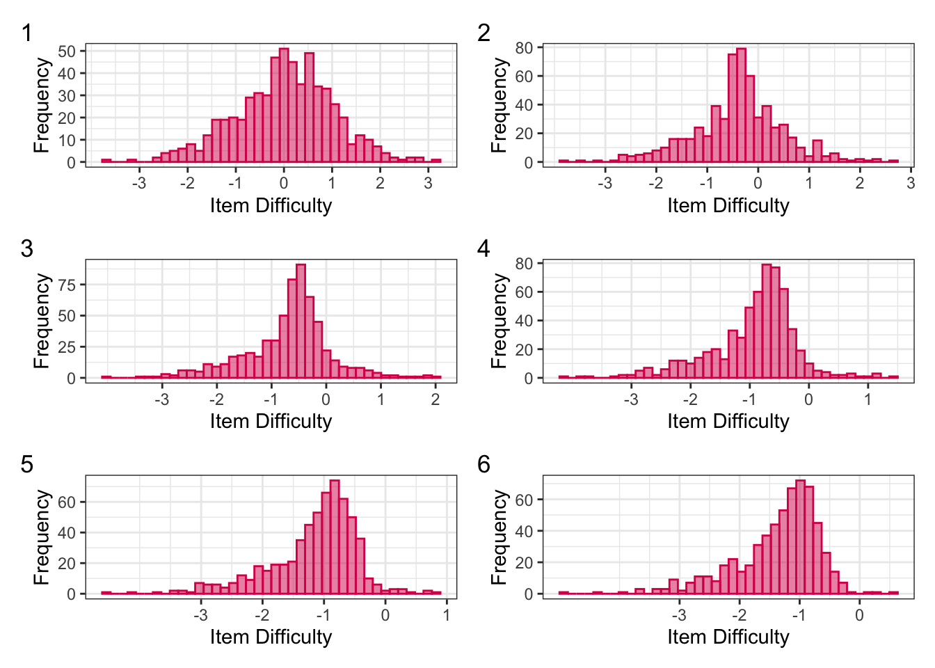
Figure 1 presents the distributions of our item difficulty values at each of the six time points. At each time point, you can see the item difficulty values shift left, indicating that they have become easier over time.
item_difficulty_distributions <-
  lapply(item_difficulty_study, function(beta_value) {
    data.table(
      beta_value = beta_value
      ) |>
      ggplot(aes(x = beta_value)) +
      geom_histogram(
        alpha = .5,
        bins = 40,
        colour = "#d81159",
        fill = "#d81159"
      ) +
      theme_bw() +
      labs(
        x = "Item Difficulty",
        y = "Frequency"
      ) +
      scale_x_continuous(
        breaks = -3:3 * 1
      )
})

wrap_plots(
  item_difficulty_distributions,
  byrow = T,
  ncol = 2) +
  plot_annotation(tag_levels = 1)
Computerised Adaptive Test Design
All our simulations will use the same CAT design so we can see the effects of item drift. It’s more detailed than the previous post, but the irt package makes this straightforward.
IP is the item pool. In our case, it is based on our 600 item difficulty values simulated above.
First item rule determines what item an examinee receives first. In our case, it is based on a fixed ability value of 1. This means that a random question with a difficulty value of 1 will be selected. An alternative approach would be randomly selecting an ability value from a specified ranged.
Three test termination criteria are set. The examinee needs to have completed, at a minimum, 15 questions in the CAT. At most, they answer 25 questions. Between 15 and 25 questions, the CAT can end early if the ability estimate error is less than .2.
The next question selection uses the randomesque method. So from the number of most informative items specified (in this case five), one item is randomly selected.
I’ve wrapped this in a function as part of the CAT simulation so for each iteration it is passed the updated item difficulty values.
cat_study_design <- function(item_bank) {
  create_cat_design(
    ip = item_bank,
    title = "Item Drift Study",
    first_item_rule = "fixed_theta",
    first_item_par = list(
      theta = 1
    ),
    next_item_rule = "mfi",
    ability_est_rule = "ml",
    final_ability_est_rule = "ml",
    termination_rule = c("min_item", "min_se", "max_item"),
    termination_par = list(
      min_item = 15,
      min_se = .2,
      max_item = 25
    ),
    exposure_control_rule = "randomesque",
    exposure_control_par = list(
      num_items = 5
    )
  )
}
Running the Computerised Adaptive Test
To run the study, we need examinees. We don’t have that data so again we sample 1000 values from a normal distribution (Mean = 0, SD = 1).
The study is then run. Each iteration involves passing in one of the six item difficulty vectors. An itempool is created, which sets out our study items. In this cases, our items are based on the one-parameter model and labelled from item_1 to item_600.
From the study, we generate a list containing the CAT results, the item bank details, and item exposure rates.
true_ability <- rnorm(1e3, 0, 1)

cat_results <- lapply(item_difficulty_study, function(study_data) {

  item_bank <-
    itempool(
      b = study_data,
      model = "1PL",
      item_id = paste0("item_", 1:600)
    )

  cat_design <-
    cat_study_design(item_bank)

  cat_results <-
    cat_sim_fast(
      true_ability = true_ability,
      cd = cat_design,
      n_cores = 6
    )

  exposure_rates <-
    calculate_exposure_rates(
      cat_results,
      cd = cat_design
    )

  return(
    list(
      item_bank = item_bank,
      cat_output = cat_results,
      exposure_rates = exposure_rates
    )
  )

})
Simulation Results
From the simulation, we’re interested in the precision of our measures and the impact drift has had on item exposure rates.
Measurement Precision
Bias is the average difference between the true and estimated ability estimate. We can also calculate two measures of overall error: Mean Absolute Error (MAE) and Root Mean Square Error (RMSE).
cat_precision <- lapply(cat_results, function(x) {

  ability_estimates <-
    summary(x$cat_output, "true_ability", "est_ability") |>
    as.data.table()

  ability_estimates[, bias := est_ability - true_ability]

  measurement_precision <-
    ability_estimates[,
                      .(
                        bias = sum(bias) / .N,
                        mae = sum(abs(bias)) / .N,
                        rmse = sqrt((sum(bias^2) / .N))
                        )]
}) |>
  rbindlist()

cat_precision[, simulation_run := 1:nrow(cat_precision)]

cat_precision[, .(simulation_run, bias, mae, rmse)] |>
  flextable() |>
  colformat_double(digits = 3) |>
  set_header_labels(
    values = c(
      "Simulation Run",
      "Bias",
      "MAE",
      "RMSE"
    )
  ) |>
  align(
    j = 1,
    align = "center"
  ) |>
  autofit()
Simulation Run | Bias | MAE | RMSE |
|---|---|---|---|
1 | 0.010 | 0.364 | 0.456 |
2 | 0.006 | 0.351 | 0.442 |
3 | -0.006 | 0.346 | 0.438 |
4 | -0.008 | 0.350 | 0.449 |
5 | -0.001 | 0.353 | 0.453 |
6 | 0.007 | 0.382 | 0.489 |
The table shows our measurement precision. The first simulation does have more error than simulations two through five. Simulation six has the highest error, with an average difference of ~.05 between true and estimated ability values. It does suggest there is a problem somewhere, but doesn’t point to where said problem lies.
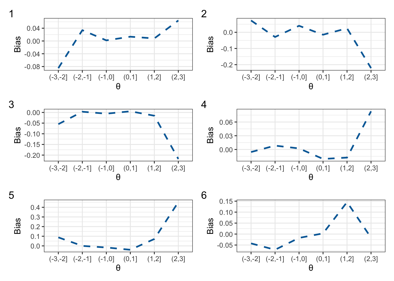
Conditional bias, however, can help identify where the problem lies. That is, we calculate the bias at different intervals along the ability scale. This is presented in Figure 2. At the first step in the simulation, the CAT underestimated abilities within the (-3, -2] interval, but overestimated abilities at the (2, 3] interval. Throughout the simulation, the fewer difficult items led to the bias estimates fluctuating highly at the (2, 3] interval relative to other ability intervals.
cat_conditional_bias <- lapply(cat_results, function(x) {

  ability_estimates <-
    summary(x$cat_output, "true_ability", "est_ability") |>
    as.data.table()

  ability_estimates[,
                    true_ability_interval := cut(true_ability,
                                                 breaks = c(-10,-4,-3,-2,-1,
                                                            0,
                                                            1, 2, 3, 4, 10)
                                                 )]

  ability_estimates[, bias :=  est_ability - true_ability]

  conditional_bias <-
    ability_estimates[,
                      .(bias = sum(bias) / .N),
                      by = true_ability_interval]

  conditional_bias |>
    ggplot(aes(x = true_ability_interval, y = bias, group = 1)) +
    geom_line(
      colour = "#006ba6",
      linejoin = "round",
      linetype = 2,
      linewidth = 1
    ) +
    theme_bw() +
    labs(
      x = "θ",
      y = "Bias"
    )

})

wrap_plots(
  cat_conditional_bias,
  byrow = T,
  ncol = 2)  +
  plot_annotation(tag_levels = 1)
Item Exposure
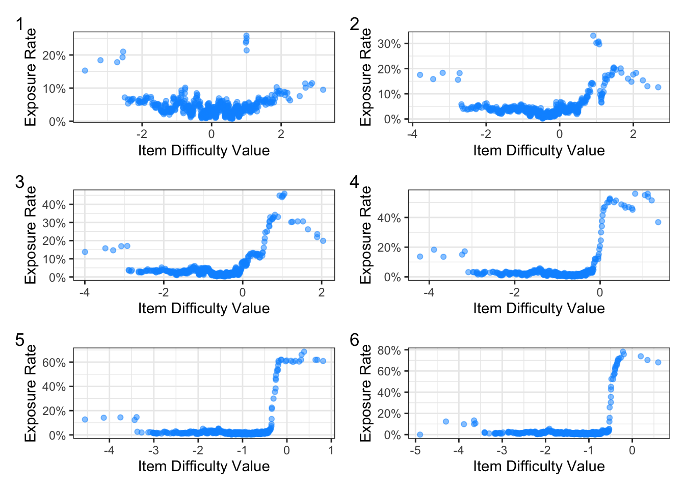
Figure 3 shows the effect of item drift on exposure rates. At the start, majority of exposure rates are less than 10%. There are a few items with exposure rates above 20%, which is due to the initial fixed ability that was set for the CAT. With each simulation run, you can see that as there are fewer difficult items, the exposure rates for the remaining items at upper-end of the ability scale exceed 40%.
difficulty_exposure_plots <- lapply(cat_results, function(x) {

  exposure_rates <-
    x$exposure_rates |>
    as.data.table(
      keep.rownames = T
    )

  setnames(
    exposure_rates,
    old = c("V1", "V2"),
    new = c("item_id", "exposure_rate")
  )

  item_details <-
    x$item_bank |>
    as.data.table()

  item_details <-
    item_details |>
    merge(
      exposure_rates,
      by = "item_id"
    )

  item_details |>
    ggplot(aes(x = b, y = exposure_rate)) +
    geom_jitter(
      alpha = .5,
      colour = "#0496ff",
      fill = "#0496ff",
      shape = 21
    ) +
    theme_bw() +
    scale_y_continuous(
      labels = percent_format()
    ) +
    labs(
      x = "Item Difficulty Value",
      y = "Exposure Rate"
    )

})

wrap_plots(
  difficulty_exposure_plots,
  byrow = T,
  ncol = 2)  +
  plot_annotation(tag_levels = 1)
Summary
Item compromise and Generative AI can have significant impact on CATs. Each can contribute to questions becoming easier to answer, which makes estimating abilities less reliable. In the context of recruitment, this could mean that we are making sifting decisions based on inaccurate measurements. That is, candidates receive ability estimates that are higher than their true ability, or estimates lower than their ability. It is necessary that item parameters are continually monitored, along with the CAT itself. Item compromise also needs to be checked to ensure that the questions and possible solutions cannot be found online.