Equating Noise: Re-Examining a GPCM Study Through Simulation

This post discusses a measurement paper that leaves a lot to be desired. The aim isn’t to criticise the authors personally, but to show the substantial problems in the analyses and highlight steps readers should avoid in their own work.

library(data.table)
library(flextable)
library(ggplot2)
library(irt)
library(mirt)

Loading required package: stats4

Loading required package: lattice

Study Overview

The paper attempts to equate two test forms (A and B) designed to measure academic ability in Natural Sciences. Equating places scores from one form onto the scale of another using a small set of common “anchor items” (in this case, eight items). The remaining items are unique to each form.

A total of 281 students participated (Form A: 141; Form B: 140). Responses were modelled using the Generalized Partial Credit Model (GPCM) due to items being scored 0–3. The authors had no prior evidence that either test form was valid, reliable, or well-functioning.

Reported Model Fit

The reported fit of the GPCM models were as follows:

• Form A: TLI = .511, CFI = .549, RMSEA = .0286, SRMR = .081

• Form B: TLI = .542, CFI = .578, RMSEA = .0526, SRMR = .088

The authors conclude the RMSEA indicates “good fit” and move on with the analysis.

This is incorrect.

• TLI and CFI are far below any acceptable threshold (common cut-off is ≥ .95 for IRT models; even the most lenient standards would reject values this low).

• No χ² (or equivalent) test is provided, which is standard practice.

• RMSEA can appear artificially “good” in poorly identified models, especially when parameters are unstable or the model is oversized relative to sample size.

Taken together, the model clearly does not fit the data, and the results should not be interpreted without further investigation.

Item Parameter Problems

Below is an excerpt of Form A item parameters (10 of the 30 items).

If we use .70 as a minimum discrimination (a) value, all items fall below that threshold. One item even has a negative discrimination, meaning higher-ability students are less likely to score well, which is a red flag for misfit or miscoding.

Thresholds (b1–b3) are also severely disordered, extremely large, and inconsistent with realistic category structure. Given the poor global fit and small sample, these estimates should be treated as unreliable.

# Form A Item Bank
form_a_parameters <- 
  fread("form_a_parameters.txt")

form_a_parameters |>
  as_flextable() |>
  colformat_double(digits = 3)

Table 1: Form A item parameters

Items	a	b1	b2	b3
character	numeric	numeric	numeric	numeric
A1	0.445	3.157	0.735	-1.001
A2	0.484	1.992	-1.356	-0.206
A3	0.404	-2.737	-0.843	-5.518
A4	0.222	0.158	6.407	2.670
A5	0.222	8.335	-5.422	4.561
A6	0.112	15.022	-8.322	-4.688
A7	0.318	0.463	-0.561	-1.069
A8	0.118	11.285	0.456	17.818
A9	-0.021	-8.952	-75.053	-25.707
A10	0.197	3.462	0.803	-1.320
n: 30

The same issues appear in Form B, shown below.

# Form B Item Bank
form_b_parameters <- 
  fread("form_b_parameters.txt", fill = T)

form_b_parameters |>
  as_flextable() |>
  colformat_double(digits = 3)

Table 2: Form B item parameters

Items	A	b1	b2	b3
character	numeric	numeric	numeric	numeric
B23	0.192	-4.601	-0.125	-5.614
B24	0.376	3.462	-0.118	-0.240
B25	0.387	4.746	-3.474	2.716
B26	-0.154	-13.168	-0.184
B27	0.190	7.774	-10.433	11.886
B28	0.381	-3.562	6.557	-7.262
B29	-0.186	-11.521	4.917	-18.528
B30	0.054	14.996	10.455	16.409
B31	0.149	13.962	-18.489	12.708
B32	0.407	4.116	-4.161	4.773
n: 30

Simulation

A simulation is needed for one reason: the reported model is not trustworthy.

• The model does not fit the data.

• The item parameters are implausible and highly unstable.

• Under these conditions, equating is irrelevant, if the underlying model is noise, then equating simply aligns one set of noise to another.

To demonstrate the instability, I simulate datasets using the reported Form A GPCM parameters 1000 times and re-estimate the models. This allows us to examine:

• the spread of recovered item thresholds and discrimination estimates

• the uncertainty in model-fit indices

In other words, I show what the authors did not: the amount of uncertainty in the reported results.

set.seed(2511)

form_a_bank <-
  itempool(form_a_parameters, model = "GPCM")

simulation_results <- lapply(1:1e3, function (i) {
  resp <- sim_resp(form_a_bank, rnorm(141))
  gpcm_model <- mirt(resp, itemtype = "gpcm", verbose = F)
  
  list(
    model_fit = M2(gpcm_model),
    item_parameters = coef(gpcm_model, IRTpars = T, simplify = T)$items
  )
})

Across the 1000 replications, we replicate the findings of the author: “good” RMSEA/SRMSR paired with poor CFI/TLI (Table 3). However, the standard deviations of CFI and TLI are large, showing that the fit statistics themselves are unstable. The point estimates of the original paper are not showing the full picture: the estimates are extremely variable.

model_fit <-
  lapply(simulation_results, function (x) x$model_fit) |>
  rbindlist(fill = T)

model_fit[, .(
  "Fit Measure" = names(.SD),
  "Mean" = apply(.SD, 2, function(x) mean(x, na.rm = T)), 
  "SD" = apply(.SD, 2, function(x) sd(x, na.rm = T))), 
  .SDcols = c("RMSEA", "SRMSR", "TLI", "CFI")] |>
  as_flextable() |>
  colformat_double(digits = 3)

Table 3: Model fit summary from simulation study

Fit Measure	Mean	SD
character	numeric	numeric
RMSEA	0.011	0.012
SRMSR	0.076	0.003
TLI	1.007	10.580
CFI	0.678	0.363
n: 4

To visualise this, Figure 1 plots the distribution of each fit measure across replications. The spread is wide, especially for the incremental fit indices.

model_fit[, simulation_run := .I] |>
  melt(id.vars = "simulation_run", variable.name = "fit_measure") |>
  ggplot(aes(x = value)) +
  geom_histogram(
    colour = "black",
    fill = "white"
  ) +
  facet_wrap(~fit_measure, scales = "free") +
  theme_bw()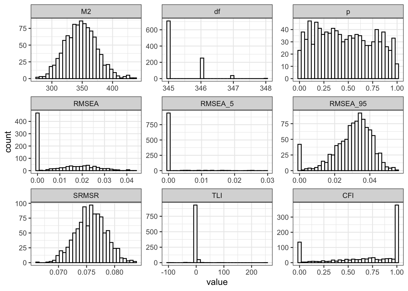

Figure 1: Fit measure distributions across simulation runs

Next, we examine the recovered item parameters. For each simulation, I extracted the re-estimated discrimination and thresholds. Table 4 summarises the mean and standard deviation per item and per parameter. The results show what the paper never reports: massive instability in several thresholds, particularly for items with already questionable estimates.

model_parameters <- 
  lapply(simulation_results, function (x) as.data.table(x$item_parameters, keep.rownames = T)) |>
  rbindlist(fill = T)

model_parameters[,
                 .(
                   "Fit Meaure" = names(.SD),
                   "Mean" = apply(.SD, 2, function (x) mean(x, na.rm = T)),
                   "SD" = apply(.SD, 2, function (x) sd(x, na.rm = T))
                 ),
                 by = c("Item ID" = "rn"),
                 .SDcols = c("a", "b1", "b2", "b3")] |>
  as_flextable(max_row = 20) |>
  colformat_double(digits = 3)

Table 4: Item parameter simulation summary

Item ID	Fit Meaure	Mean	SD
character	character	numeric	numeric
Item_1	a	0.465	0.154
Item_1	b1	3.478	1.564
Item_1	b2	0.756	1.038
Item_1	b3	-1.151	1.123
Item_2	a	0.505	0.158
Item_2	b1	2.137	1.124
Item_2	b2	-1.438	0.878
Item_2	b3	-0.271	0.643
Item_3	a	0.428	0.199
Item_3	b1	-3.382	4.758
Item_3	b2	-1.182	4.546
Item_3	b3	-7.381	13.477
Item_4	a	0.226	0.131
Item_4	b1	0.563	11.962
Item_4	b2	18.475	259.597
Item_4	b3	9.416	148.147
Item_5	a	0.234	0.118
Item_5	b1	-1.276	282.750
Item_5	b2	1.751	203.804
Item_5	b3	-3.691	235.424
n: 120

The pattern is clear:

• Discriminations show modest variability.

• Thresholds for several items explode, sometimes with SDs in the hundreds.

• This confirms that the original parameter estimates are not stable enough to support equating.

Summary

The results reported in the paper cannot be trusted. The model does not fit, the item parameters are unstable, and the equating is performed on foundations that do not hold.

Before any equating could be justified, the authors should have validated the scale, checked dimensionality, examined category functioning, and ensured item quality. None of this was done. Instead, the analysis proceeds on the basis of a single favourable RMSEA value, while the remaining fit indices clearly reject the model.

The sample size is insufficient for the complexity of the model, many items behave pathologically, and there is no evidence that the test measures a single latent trait.

The simulation demonstrates what the paper did not: the estimates are highly unstable, the fit indices vary widely, and the recovered parameters exhibit enormous uncertainty. The published results give a false impression of precision.

As it stands, the findings are not interpretable and the paper’s conclusions are unsupported.