library(data.table)
library(flextable)
library(ggplot2)
library(lavaan)
library(patchwork)
library(responsePatterns)
library(semPlot)

grit_data <-
fread("data/data.csv")As a Psychometrician, my role involves the analysis of questionnaires. Why? Because we need to know if we are measuring what we say we measure!
So in this post, we look to ‘psychometrically’ analyse data about Grit.
Grit is a personality trait that has had been quite popular, resulting in various books and TedTalks, but like anything popular, it’s not exempt from criticism.
Analysing Psychometric Data
Time Spent on the Survey
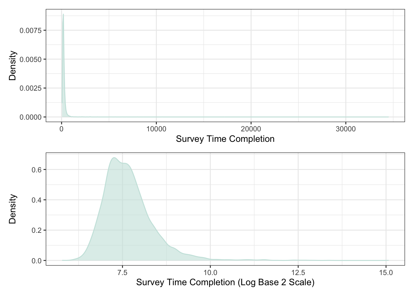
With any questionnaire data, you should start by checking how long it took an individual to complete the survey itself. This can be achieved by visualising the distributions, as in Figure 1. It’ll become immediately apparent from the top panel that it is difficult to visualise what’s going on. This is because there are individuals in the data who spent over 10,000 seconds (~3 hours) on 62 item questionnaire. It’s doubtful that anyone taking a survey would spend so much time out of their day to complete it. The likelihood is that the individual stepped away mid-way through the survey and returned to complete it a later point in time.
To improve the presentation and make it clearer, we can re-scale the x-axis by converting the values to the Log Base 2 scale. The bottom panel illustrates the transformation, which has allowed us to see the distribution. To find the inverse of any number on the x-axis, raise 2 to the power of the associated x value. For example 2^7.5 = 181 seconds.
survey_time <-
  ggplot(grit_data, aes(x = surveyelapse)) +
  geom_density(
    alpha = .6,
    colour = "#C9E4DE",
    fill = "#C9E4DE"
  ) +
  labs(
    x = "Survey Time Completion",
    y = "Density"
  ) +
  theme_bw()

survey_time_logtwo <-
  ggplot(grit_data, aes(x = log2(surveyelapse))) +
  geom_density(
    alpha = .6,
    colour = "#C9E4DE",
    fill = "#C9E4DE"
  ) +
  labs(
    x = "Survey Time Completion (Log Base 2 Scale)",
    y = "Density"
  ) +
  theme_bw()

survey_time / survey_time_logtwo
Given the presence of a few long survey completion times, summary statistics should be robust to potential outliers. Therefore, we use medians and median absolute deviations (MADs) instead of means and standard deviations. Below is a table summarising these statistics:
Median completion time: 189 seconds (~3 minutes)
Median absolute deviation: 74.1 seconds
This means that half of the respondents completed the survey in less than 189 seconds, and half took longer. The MAD indicates that typical completion times deviated from the median by about 74.1 seconds.
How do we proceed?
The maximum completion time was 34522 seconds (~10 hours). This may indicate a careless respondent, although additional information may be required to make such assertions (e.g., inspect response patterns).
Response Patterns
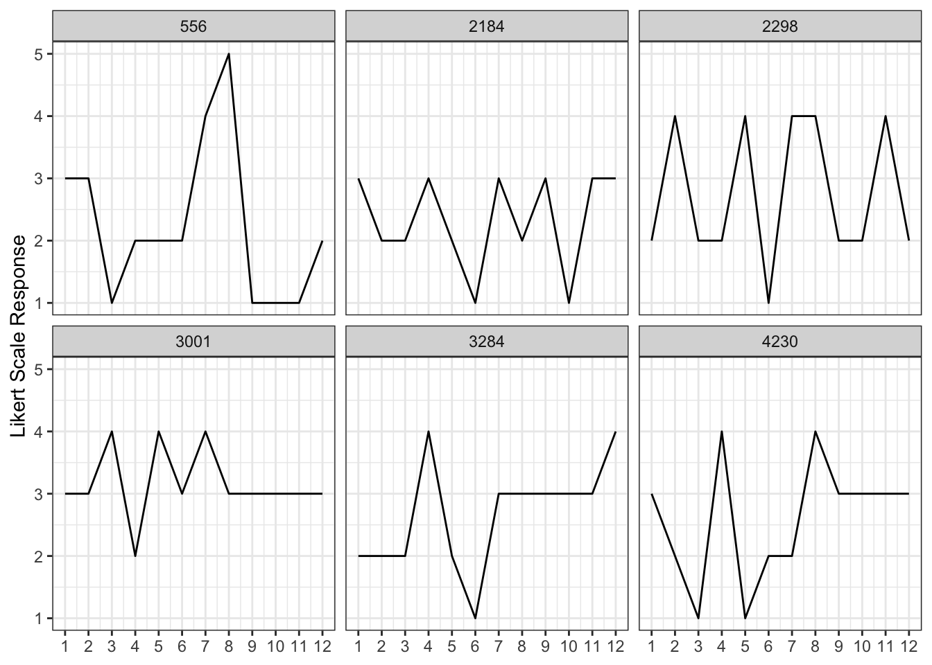
Let’s take a quick detour! I recently discovered the responsePatterns R package, which offers a clever way to identify potentially careless survey responses. It uses autocorrelations to detect patterns in how people answer items. Take a look at Figure 2 – each plot shows an individual respondent. Notice how respondent 3001 starts selecting the middle response from item 8 onwards. This pattern, along with other evidence like unusually short response times, could suggest careless responding. It’s important to use this kind of evidence carefully and document your decisions when considering whether to exclude any participants from your analysis.
set.seed(25022024)

# Use Response Pattern Package to calculate Autocorrelations

grit_autocorrelations <-
  rp.acors(grit_data[, .SD, .SDcols = patterns("^GS")])
max.lag automatically set to 9percentile_select <-
rp.select(grit_autocorrelations, percentile = 85)
# Subset of Rows based on Autocorrelation Indices
percentile_select_index <-
as.numeric(row.names(percentile_select@indices)) |>
sample(size = 6)
grit_subset_data <-
grit_data[percentile_select_index, .SD, .SDcols = patterns("^GS")]
grit_subset_data <-
grit_subset_data[, index := percentile_select_index] |>
melt(
id.vars = "index"
)
grit_subset_data[, variable := as.numeric(gsub("GS", "", variable))]
# Plot Response Patterns
ggplot(grit_subset_data, aes(x = variable, y = value, group = index)) +
geom_path() +
facet_wrap(~index) +
labs(
x = NULL,
y = "Likert Scale Response"
) +
theme_bw() +
scale_x_continuous(
breaks = 1:12*1
)
Evaluating Models
When applying psychometric methods, a common starting point is exploratory factor analysis (EFA). This helps us refine our understanding of a questionnaire or test by uncovering the underlying structure of the items. This ‘factor structure’ refers to the groups of related items that seem to measure broader concepts or traits. For example, we might find that a subset of questions measures the personality trait of Openness, while another subset relates to Agreeableness. EFA can be a valuable way to start organising the data and identify potential theoretical concepts.
Often, researchers will follow up with confirmatory factor analysis (CFA). In CFA, we use a new dataset to test whether a structure suggested by EFA actually fits the pattern of responses well. While CFA involves statistical evaluation, it’s a way to refine and validate our theoretical understanding of a measure.
The 12 items from the original Grit Scale are presented in the table below. Previous work has already identified a two factor structure of Consistency of Interests and Perseverance of Effort. Each being measured by six items. Responses were captured on a 5-point Likert Scale ranging from Very Much Like Me (1) to Not Like Me at All (5).
| Item Code | Item/Statement | Measures |
|---|---|---|
| GS1 | I have overcome setbacks to conquer an important challenge. | Perseverance of Effort |
| GS2 | New ideas and projects sometimes distract me from previous ones. | Consistency of Interest |
| GS3 | My interests change from year to year. | Consistency of Interest |
| GS4 | Setbacks do not discourage me. | Perseverance of Effort |
| GS5 | I have been obsessed with a certain idea or project for a short time but later lost interest. | Consistency of Interest |
| GS6 | I am a hard worker. | Perseverance of Effort |
| GS7 | I often set a goal but later choose to pursue a different one. | Consistency of Interest |
| GS8 | I have difficulty maintaining my focus on projects that take more than a few months to complete. | Consistency of Interest |
| GS9 | I finish what I begin. | Perseverance of Effort |
| GS10 | I have achieved a goal that took years of work. | Perseverance of Effort |
| GS11 | I become interested in new pursuits every few months. | Consistency of Interest |
| GS12 | I am diligent. | Perseverance of Effort |
Testing Various Models
The authors of the Grit Scale proposed a specific two-factor structure. Here, we’ll investigate this question further by comparing two different models of the scale’s underlying structure:
CFA Representation: This is a stricter model where each item loads onto only a single factor and we do not allow for correlated errors (this assumes item wording is completely distinct).
EFA Representation: This is more flexible, allowing items to potentially load onto multiple factors (cross-loadings). This is useful if some items seem to measure more than just one dimension of grit. We still don’t include correlated errors.
By comparing the fit of these two models, we can gain insights into the degree to which the Grit Scale items cleanly separate into just two factors, or if a more nuanced understanding of the constructs is needed.
CFA Representation
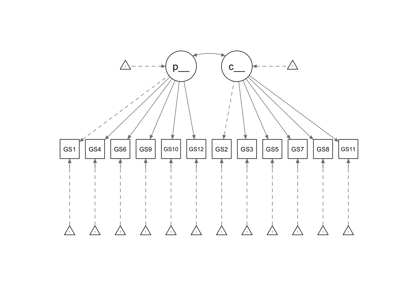
Figure 3 illustrates the relationships between the factors we’re exploring and the specific questions designed to measure them. This type of diagram, called a Confirmatory Factor Analysis (CFA), uses reflective measurements. This means we theorise that changes in the underlying factors (like consistency of interest) will be reflected in how people answer the related survey questions. Let’s use the familiar example of depression to make this clearer. As a construct, it is not directly observable. It manifests in various ways (e.g., difficulty sleeping and irritability). If depression worsened, then we would see changes in these symptoms (i.e., they get worse). Whereas, an improvement in depression would, in most cases, reduce the severity of such symptoms. In other words, we use the symptoms as measures of the underlying construct (depression).
grit_cfa_model <- "
  perseverance_of_effort =~ GS1 + GS4 + GS6 + GS9 + GS10 + GS12
  consistency_of_interest =~ GS2 + GS3 + GS5 + GS7 + GS8 + GS11
"

grit_cfa_fit <-
  cfa(
    grit_cfa_model,
    grit_data,
    ordered = TRUE
  )

semPaths(
  grit_cfa_fit,
  what = "diagram",
  style = "lisrel",
  thresholds = F)
Inspecting Item Loadings
The Table below presents the loadings for each item onto its respective factor. Ideally, we want factor loadings to be large (exceeding an absolute value of .4) to indicate that an item is a strong measure of the underlying concept. In general, the loadings look acceptable. GS4 has the lowest loading of .4, followed by GS11 (loading of .47). While these are still within an acceptable range, it might suggest room for further refining these items in the future.
grit_cfa_loadings <-
  parameterestimates(grit_cfa_fit, standardized = T) |>
  as.data.table()

grit_cfa_loadings[op == "=~", .(lhs, op, rhs, est, se, std.all)] |>
  _[, lhs := ifelse(
    lhs == "perseverance_of_effort",
    "Perseverance of Effort",
    "Consistency of Interest")] |>
  flextable() |>
  merge_at(
    i = 1:6,
    j = 1
  ) |>
  merge_at(
    i = 7:12,
    j = 1
  ) |>
  merge_at(
    i = 1:12,
    j = 2
  ) |>
  colformat_double(
    digits = 2
  ) |>
  fix_border_issues() |>
  hline(i = 6, j = 3:6) |>
  set_header_labels(
    values = c(
      "Factor",
      "Operation",
      "Item",
      "Unstandardised Estimate",
      "Standard Error",
      "Standardised Estimate")
  ) |>
  align_nottext_col(
    align = "center"
  ) |>
  set_caption(
    "Factor loadings obtained from the Two-Factor Confirmatory Factor Model of the 12-item Grit scale."
  )
Factor | Operation | Item | Unstandardised Estimate | Standard Error | Standardised Estimate |
|---|---|---|---|---|---|
Perseverance of Effort | =~ | GS1 | 1.00 | 0.00 | 0.55 |
GS4 | 0.72 | 0.03 | 0.40 | ||
GS6 | 1.33 | 0.03 | 0.73 | ||
GS9 | 1.48 | 0.03 | 0.81 | ||
GS10 | 1.24 | 0.03 | 0.68 | ||
GS12 | 1.27 | 0.03 | 0.70 | ||
Consistency of Interest | GS2 | 1.00 | 0.00 | 0.61 | |
GS3 | 1.02 | 0.02 | 0.63 | ||
GS5 | 1.21 | 0.02 | 0.74 | ||
GS7 | 1.29 | 0.02 | 0.79 | ||
GS8 | 1.34 | 0.02 | 0.82 | ||
GS11 | 0.76 | 0.02 | 0.47 |
Inspecting the Global Fit
Now that we’ve looked at individual item loadings, let’s assess how well the model as a whole fits the data. There are various “goodness-of-fit” measures for this. To simplify things, we’ll focus on a few key ones: Chi-Square, CFI, TLI, RMSEA, and SRMR. Unfortunately, our model doesn’t show a perfect fit based on the Chi-Square test. While there’s debate on the importance of this specific test, other measures suggest a decent fit. Still, this mismatch might mean we need to explore different model structures. The alternative fit measures show the model to have an acceptable fit. For our purposes, we’ll assume the model is correct and carry on.
fitmeasures(
  grit_cfa_fit,
  fit.measures = c(
     "chisq",
     "df",
     "pvalue",
     "cfi",
     "tli",
     "rmsea",
     "srmr"), output = "matrix"
  ) |>
  as.data.table(
    keep.rownames = TRUE
  ) |>
  flextable() |>
  colformat_double(
    digits = 2
  ) |>
  set_caption(
    caption = "Loadings obtained from the two-factor Confirmatory Factor Analysis model."
  ) |>
  set_header_labels(
    values = c("Fit Measure", "Value")
  )
Fit Measure | Value |
|---|---|
chisq | 2,532.54 |
df | 53.00 |
pvalue | 0.00 |
cfi | 0.96 |
tli | 0.95 |
rmsea | 0.10 |
srmr | 0.07 |
Inspecting Residuals
Let’s dive deeper and examine “local fit” – how closely our model matches the relationships between individual items. The residual matrix highlights places where the model doesn’t align perfectly with the data. For instance, GS1 (“I have overcome setbacks...”) seems to have unusually strong connections with several other items (GS2, GS3, GS4, and GS11). This might be due to similar wording about overcoming challenges, suggesting there’s some overlap we could address to shorten the survey.
For example, GS1 refers to overcoming setbacks to address a challenge, as does GS4. So there’s an overlap in content. Both items reference setbacks and not seeing them as a challenge. Therefore, individual are more than likely responding the same way to both items, meaning that one item could easily be dropped, and we could then shorten the questionnaire.
The connection between GS1 and items like GS4 is obvious due to similar wording. However, the link with GS2, GS3, and GS11 requires a closer look. What we need to do is re-frame GS1. GS1 could be viewed as asking if the individual continues with an important challenge in their life, despite the challenges they face. In this way, the important challenge is viewed as an interest and it remains consistent, despite challenges. This suggests that GS1 might actually measure both Perseverance of Effort and Consistency of Interest.
rn | GS1 | GS4 | GS6 | GS9 | GS10 | GS12 | GS2 | GS3 | GS5 | GS7 | GS8 | GS11 |
|---|---|---|---|---|---|---|---|---|---|---|---|---|
GS1 | ||||||||||||
GS4 | 0.15 | |||||||||||
GS6 | 0.07 | -0.01 | ||||||||||
GS9 | -0.09 | -0.02 | -0.07 | |||||||||
GS10 | 0.09 | 0.00 | -0.05 | -0.05 | ||||||||
GS12 | 0.05 | 0.01 | 0.11 | -0.08 | -0.04 | |||||||
GS2 | 0.12 | 0.03 | 0.05 | -0.10 | 0.02 | 0.04 | ||||||
GS3 | 0.11 | 0.10 | 0.09 | 0.03 | 0.02 | 0.05 | 0.02 | |||||
GS5 | 0.07 | 0.04 | 0.04 | -0.11 | -0.02 | 0.01 | 0.02 | 0.04 | ||||
GS7 | 0.05 | 0.03 | 0.05 | -0.10 | -0.02 | 0.03 | -0.01 | 0.02 | -0.01 | |||
GS8 | 0.01 | -0.05 | -0.03 | -0.17 | -0.16 | -0.02 | -0.01 | -0.08 | -0.06 | -0.02 | ||
GS11 | 0.20 | 0.13 | 0.12 | 0.07 | 0.10 | 0.15 | 0.03 | 0.20 | 0.04 | 0.06 | -0.06 |
EFA Representation
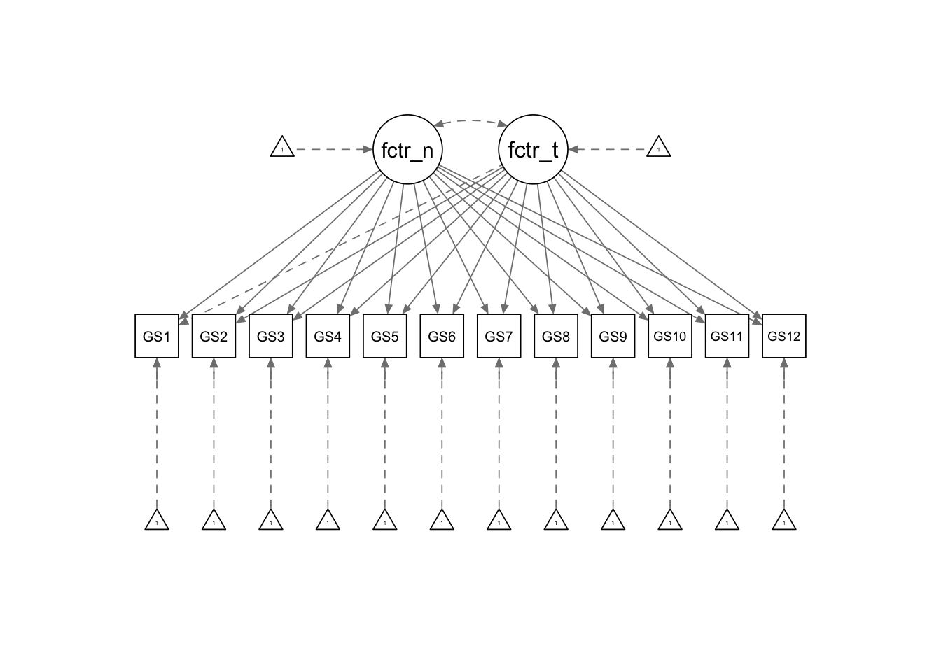
Figure is our Exploratory Factor Analysis model (Figure 4). Unlike the CFA, here we acknowledge that our survey items measure multiple factors, also known as cross-loadings. Ideally, we’d want our measures to perfectly define a single factor, but in practice, this isn’t always the case. Our model specification is slightly different here. We specify two factors, but allow all 12 items to freely load onto them. In doing so, we have forgone the labels of Perseverance of Effort and Consistency of Interests for Factor One and Factor Two.
grit_efa_model <- "
  efa('efa1')*factor_one +
  efa('efa1')*factor_two =~ GS1 + GS2 + GS3 + GS4 +
  GS5 + GS6 + GS7 + GS8 + GS9 + GS10 + GS11 + GS12
"

grit_efa_fit <-
  cfa(
    grit_efa_model,
    grit_data,
    ordered = TRUE
  )

semPaths(
  grit_efa_fit,
  what = "diagram",
  style = "lisrel",
  thresholds = F)
Inspecting Item Loadings
The EFA model loadings are shown below. Most items load highly on their theorised factors, a positive sign. However, GS4 remains an issue with a weak loading. Additionally, GS9 and GS11 exhibit moderate cross-loadings, suggesting they may measure aspects of both factors.
grit_efa_loadings <-
  parameterestimates(grit_efa_fit, standardized = T) |>
  as.data.table()

grit_efa_loadings[op == "=~", .(lhs, op, rhs, est, se, std.all)] |>
  _[, lhs := ifelse(
    lhs == "factor_one",
    "Factor One",
    "Factor Two")] |>
  flextable() |>
  merge_at(
    i = 1:12,
    j = 1
  ) |>
  merge_at(
    i = 13:24,
    j = 1
  ) |>
  merge_at(
    i = 1:24,
    j = 2
  ) |>
  colformat_double(
    digits = 2
  ) |>
  fix_border_issues() |>
  hline(i = 12, j = 3:6) |>
  set_header_labels(
    values = c(
      "Factor",
      "Operation",
      "Item",
      "Unstandardised Estimate",
      "Standard Error",
      "Standardised Estimate")
  ) |>
  align_nottext_col(
    align = "center"
  ) |>
  set_caption(
    "Factor loadings obtained from the Two-Factor Exploratory Factor Model of the 12-item Grit scale."
  )
Factor | Operation | Item | Unstandardised Estimate | Standard Error | Standardised Estimate |
|---|---|---|---|---|---|
Factor One | =~ | GS1 | 0.12 | 0.02 | 0.12 |
GS2 | 0.62 | 0.01 | 0.62 | ||
GS3 | 0.74 | 0.01 | 0.74 | ||
GS4 | 0.05 | 0.02 | 0.05 | ||
GS5 | 0.72 | 0.01 | 0.72 | ||
GS6 | -0.01 | 0.01 | -0.01 | ||
GS7 | 0.76 | 0.01 | 0.76 | ||
GS8 | 0.64 | 0.01 | 0.64 | ||
GS9 | -0.32 | 0.01 | -0.32 | ||
GS10 | -0.15 | 0.02 | -0.15 | ||
GS11 | 0.69 | 0.01 | 0.69 | ||
GS12 | -0.02 | 0.01 | -0.02 | ||
Factor Two | GS1 | 0.69 | 0.01 | 0.69 | |
GS2 | 0.00 | 0.01 | 0.00 | ||
GS3 | 0.14 | 0.02 | 0.14 | ||
GS4 | 0.47 | 0.02 | 0.47 | ||
GS5 | -0.05 | 0.02 | -0.05 | ||
GS6 | 0.76 | 0.01 | 0.76 | ||
GS7 | -0.06 | 0.02 | -0.06 | ||
GS8 | -0.25 | 0.02 | -0.25 | ||
GS9 | 0.54 | 0.01 | 0.54 | ||
GS10 | 0.59 | 0.01 | 0.59 | ||
GS11 | 0.29 | 0.02 | 0.29 | ||
GS12 | 0.71 | 0.01 | 0.71 |
Inspecting the Global Fit
Has our global fit improved? Absolutely! Our fit measures show noticeable gains. This is likely because we relaxed the strict constraint of items loading onto only one factor. Despite this improvement, the Chi-Square test remains significant, suggesting our model might not perfectly represent the data.
fitmeasures(
  grit_efa_fit,
  fit.measures = c(
     "chisq",
     "df",
     "pvalue",
     "cfi",
     "tli",
     "rmsea",
     "srmr"), output = "matrix"
  ) |>
  as.data.table(
    keep.rownames = TRUE
  ) |>
  flextable() |>
  colformat_double(
    digits = 2
  ) |>
  set_caption(
    caption = "Global Fit Measures from the Two-Factor Exploratory Factor Analysis model."
  ) |>
  set_header_labels(
    values = c("Fit Measure", "Value")
  ) |>
  autofit()
Fit Measure | Value |
|---|---|
chisq | 448.68 |
df | 43.00 |
pvalue | 0.00 |
cfi | 0.99 |
tli | 0.99 |
rmsea | 0.05 |
srmr | 0.03 |
Inspecting Residuals
In-line with the global fit improvement, our local fit has also improved. The model still doesn’t exactly fit our data, which we know from the Chi-Square test. You can still see that various items contribute to the misfit between model and data more than others (e.g., GS4). Again, further exploration into the reasoning behind this would be important.
rn | GS1 | GS2 | GS3 | GS4 | GS5 | GS6 | GS7 | GS8 | GS9 | GS10 | GS11 | GS12 |
|---|---|---|---|---|---|---|---|---|---|---|---|---|
GS1 | ||||||||||||
GS2 | 0.04 | |||||||||||
GS3 | -0.04 | -0.02 | ||||||||||
GS4 | 0.08 | -0.01 | 0.02 | |||||||||
GS5 | 0.00 | 0.02 | 0.01 | 0.00 | ||||||||
GS6 | -0.01 | 0.01 | -0.03 | -0.06 | 0.01 | |||||||
GS7 | -0.02 | -0.01 | -0.01 | -0.00 | -0.00 | 0.02 | ||||||
GS8 | 0.03 | 0.03 | -0.05 | -0.02 | -0.02 | 0.04 | 0.03 | |||||
GS9 | -0.05 | -0.04 | 0.06 | 0.01 | -0.02 | -0.00 | -0.00 | -0.02 | ||||
GS10 | 0.06 | 0.03 | -0.01 | -0.01 | 0.01 | -0.05 | 0.02 | -0.05 | 0.02 | |||
GS11 | -0.01 | -0.04 | 0.07 | 0.01 | -0.02 | -0.06 | -0.00 | -0.04 | 0.04 | 0.01 | ||
GS12 | -0.03 | 0.01 | -0.05 | -0.04 | -0.01 | 0.06 | 0.01 | 0.05 | -0.01 | -0.04 | -0.02 |
Conclusion
Our comparison of the CFA and EFA representations of the Grit Questionnaire highlights the limitations of overly restrictive models like CFA. EFA, by allowing for cross-loadings, improved the model’s fit. If you must choose between representations, remember the principle of parsimony: simpler models (like CFA) are generally preferred. However, targeted EFA offers a flexible middle ground between purely exploratory and confirmatory approaches.
Recommendations
When a model doesn’t perfectly fit the data, consider these steps: (1) re-evaluate items with high residuals, (2) explore other model structures, (3) if possible, collect more data. Prioritise simpler models and use strong evidence to justify any changes.