# Libraries ----------------------------------
library(data.table)
library(flextable)
library(ggplot2)
library(irt)
library(mirt)
library(patchwork)Introduction
Patient Reported Outcome Measures, or PROMs, put the power of evaluation directly into patients' hands, allowing them to assess their own well-being and symptoms without relying solely on clinicians. These tools have become central in healthcare, especially as patient-centered care gains momentum.
Since 2010, the COSMIN (COnsensus-based Standards for the selection of health Measurement INstruments) initiative has worked to set the gold standard for assessing health measurement tools like PROMs. One major outcome of this effort was a checklist—the COSMIN checklist—which highlights the importance of using robust statistical methods such as Item Response Theory (IRT) for validating measurement scales.
About the Scale
In this post, the Overall Disability scale for Polyneuropathy, Organomegaly, Endocrinopathy, Monoclonal protein, and Skin changes syndrome (POEMS) is evaluated through simulations. [The paper is available here.]
The scale was developed using responses from 49 patients. Initially, the authors had a 146-item bank. Each item was rated on a 3-point scale: 0 (not possible to perform), 1 (possible, but with some difficulty), 2 (possible, without any difficulty); this order has been reversed in this post. The collected data were analysed using Partial Credit Modelling, in which item discrimination values are held constant (at a value of 1) and item thresholds are freely estimated.
Estimation Challenges
The original analysis was constrained by sample size. For a typical Rasch analysis, the sample of 49 falls below commonly recommended thresholds. Therefore, this post uses simulations to evaluate the variability in the original parameters, to determine if the original results might be questionable.
Item parameters are found in Figure 6 of the paper. Unfortunately, the thresholds are presented only in a plot that even LLMs can't extract… 😅 So, using a ruler, I've approximated the thresholds between each response category (see Table 1). This means that, in addition to any fluctuations across simulations, there is error introduced through my (hopefully decent) ability to use a ruler.
An initial concern is the range of threshold locations: they span from approximately -7 to 6.2 on the latent scale. Most texts recommend items target the range [-3, 3]. This could indicate estimation problems due to the small sample size.
# Setup Item Parameters for Simulation -------
item_parameters <-
  fread("poems_pcm.csv")

prom_item_pool <-
  itempool(
    item_parameters,
    model = "PCM")

item_parameters |>
as_flextable(max_row = 23)item | a | b1 | b2 |
|---|---|---|---|
character | integer | numeric | numeric |
take_lift | 1 | -4.0 | -2.0 |
car | 1 | -7.0 | 1.9 |
zip | 1 | -4.0 | -1.0 |
rucksack | 1 | -4.1 | -0.5 |
indoors | 1 | -4.5 | 1.0 |
gp | 1 | -3.5 | 0.2 |
shoes | 1 | -3.0 | 1.5 |
dusting | 1 | -2.0 | 0.5 |
upper_window | 1 | -1.2 | 0.5 |
stand_15min | 1 | -2.8 | 1.8 |
rubbish | 1 | -1.5 | 1.5 |
stairs | 1 | -2.5 | 2.0 |
laces | 1 | -1.2 | 1.0 |
tray | 1 | -1.8 | 2.2 |
sheets | 1 | 1.0 | 3.0 |
walk_1km | 1 | -1.0 | 2.9 |
uneven_ground | 1 | -1.0 | 3.5 |
heavy_object | 1 | 0.0 | 2.8 |
toes | 1 | -0.5 | 3.0 |
kneel | 1 | 0.3 | 3.5 |
one_leg | 1 | 1.0 | 4.5 |
standing_long | 1 | 2.0 | 5.0 |
jump | 1 | 2.2 | 6.2 |
n: 23 | |||
Simulation Setup
To run the simulation, we specify the following:
23 items
A vector of ability estimates sampled from a normal distribution (Mean: 0, SD: 1)
The number of repetitions (250)
Matrices capturing the difference between estimated threshold and ability values and their true parameter values.
# Simulation Parameters ----------------------
n_items <- length(prom_item_pool$item)
theta <- rnorm(1e3, 0, 1)
n_repetitions <- 250
simulation_results <- vector("list", length = n_repetitions)

item_b1_bias_mat <- matrix(NA, nrow = n_repetitions, ncol = n_items)
item_b2_bias_mat <- matrix(NA, nrow = n_repetitions, ncol = n_items)

theta_bias_mat <- matrix(NA, nrow = n_repetitions, ncol = length(theta))

for (i in 1:n_repetitions) {

  # Generate Response Data
  simulated_responses <-
    sim_resp(prom_item_pool, theta = theta)

  # Run PCM Model
  mod <- mirt(simulated_responses, itemtype = "Rasch", verbose = F)
  simulation_results[[i]] <- mod

  # Item Parameters: Threshold 1
  b1_est_items <- coef(mod, IRTpars = T, simplify = TRUE)$items[, "b1"]
  if (length(b1_est_items) == n_items) {
    # Difference in estimated and true threshold estimates
    item_b1_bias_mat[i,] <-
      b1_est_items - prom_item_pool$b1
  }

  # Item Parameters: Threshold 2
  b2_est_items <-
    coef(mod, IRTpars = T, simplify = TRUE)$items[, "b2"]
  if (length(b2_est_items) == n_items) {
    # Difference in estimated and true threshold estimates
    item_b2_bias_mat[i, ] <-
      b2_est_items - prom_item_pool$b2
  }

  # Bias in Ability Estimates
  est_theta <- fscores(mod, method = "EAP")
  if (length(est_theta) == length(theta)) {
    # Difference in estimated and true ability estimates
    theta_bias_mat[i,] <- est_theta - theta
  }

}
Item Parameter Bias
For each simulation run, the bias (difference between true and estimated parameter values) was calculated. To summarise, the Mean Absolute Difference (MAD) is calculated.
It is clear that there is a problem with the estimated thresholds. The MAD is notably large for those items at the extreme ends of the latent continuum. This is further shown in Figure 1. It suggests that the original threshold estimates are uncertain. It is likely that these response option categories are unlikely to be selected.
mad_b1 <- round(colMeans(abs(item_b1_bias_mat), na.rm = T), 2)
mad_b2 <- round(colMeans(abs(item_b2_bias_mat), na.rm = T), 2)

mad_thresholds <-
  rbind(mad_b1, mad_b2) |>
  as.data.table()

setnames(
  mad_thresholds,
  old = colnames(mad_thresholds),
  new = item_parameters$item
)

mad_thresholds[, item_parameter := c("b1", "b2")]

mad_thresholds |>
  melt(id.vars = "item_parameter", variable.name = "Item") |>
  dcast(Item ~ item_parameter, value.var = "value") |>
  as_flextable(max_row = 23, show_coltype = F) |>
  colformat_double(digits = 2)
Item | b1 | b2 |
|---|---|---|
take_lift | 0.35 | 0.08 |
car | 0.44 | 0.06 |
zip | 0.25 | 0.07 |
rucksack | 0.24 | 0.07 |
indoors | 0.21 | 0.06 |
gp | 0.18 | 0.06 |
shoes | 0.13 | 0.08 |
dusting | 0.09 | 0.06 |
upper_window | 0.08 | 0.06 |
stand_15min | 0.11 | 0.08 |
rubbish | 0.08 | 0.07 |
stairs | 0.10 | 0.08 |
laces | 0.08 | 0.07 |
tray | 0.08 | 0.09 |
sheets | 0.07 | 0.16 |
walk_1km | 0.07 | 0.11 |
uneven_ground | 0.06 | 0.14 |
heavy_object | 0.06 | 0.12 |
toes | 0.06 | 0.12 |
kneel | 0.06 | 0.15 |
one_leg | 0.07 | 0.30 |
standing_long | 0.08 | 0.48 |
jump | 0.09 | 0.54 |
n: 23 | ||
item_b1_plot / item_b2_plot + plot_annotation(tag_levels = "a")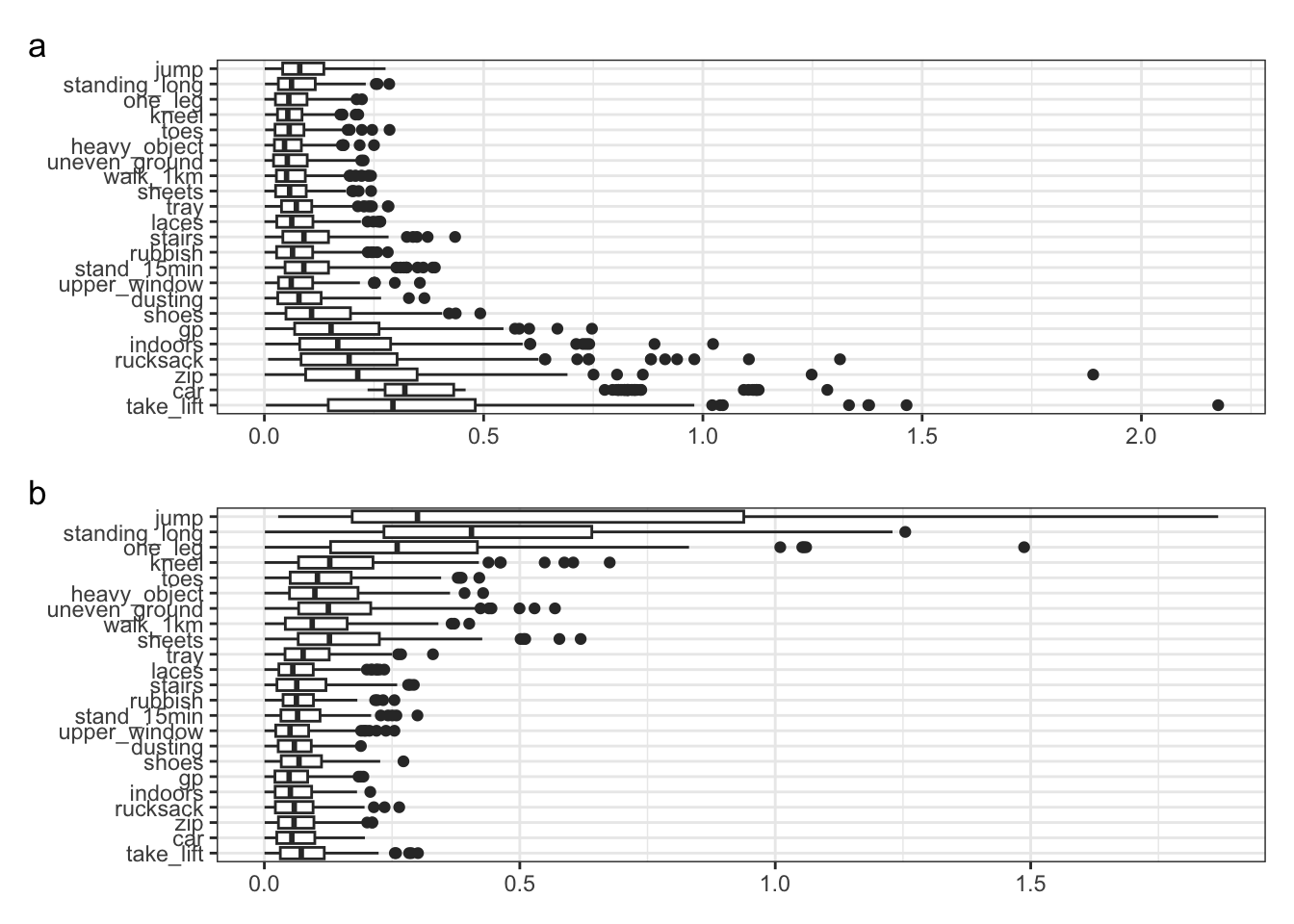
Ability Estimate Bias
mad_theta_estimate <- round(colMeans(abs(theta_bias_mat), na.rm = T), 2)The mean MAD was 0.32, which suggests that the ability estimates derived from this scale exhibit substantial uncertainty. This is a concern as estimates are off by a third of a standard deviation. In practical terms, this could lead to misclassification of their outcomes, assuming they are doing better than they are in reality.
Conclusions & Implications
Despite employing robust psychometric approaches, the simulation findings raise significant concerns about the reliability of the Overall Disability Scale for POEMs when estimated from a small sample (n = 49).
Key issues:
Ability estimates (θ) are imprecise, with an average error of 0.32, high enough to affect clinical decision-making or research interpretation.
Item threshold estimates are especially unreliable at the extremes, likely reflecting low or infrequently used categories, and limited information at those trait levels.
Implications for Use:
For clinicians and researchers tracking patient progress with this measure: apparent changes or differences may be measurement artefacts rather than true change.
There is a real risk of both overestimating and underestimating patient outcomes or treatment effects.
Recommendation:
Caution is warranted in interpreting individual scores or changes over time from this scale, particularly when used with small samples.
Substantial improvements in scale reliability could be made by increasing sample size, refining item content to ensure better targeting and use of all categories, or both.