When Perfect Fit Isn’t Perfect: Rethinking a Trace-Data SEM
This post critically examines a published path analysis linking trace data to self-regulated learning processes. It highlights issues in the model’s specification and parameterisation, and discusses the implications of these problems for interpreting trace-based measures.
SEM
Learning Analytics
Author
Alex Wainwright
Published
December 12, 2025
Learning Analytics (LA) papers have progressed: from simple event counts, to mapping log data onto presumed cognitive frameworks. But from a measurement perspective, an unresolved question remains: why does a duration of X minutes become a threshold for inferring behaviour? Time is almost always treated as a proxy for metacognition, yet its construct validity is rarely examined.
In this post, I look at a recent LA study that attempted to predict essay scores using indicators of self-regulated learning within a path model. What caught my attention was the model fit: \(\chi^2\) p-value > .05. The paper is titled: Using Trace Data of Secondary Students to Understand Metacognitive Processes in Writing From Multiple Sources.
In SEM, this is extremely rare. It implies that the model-implied covariance matrix matches the sample covariance almost perfectly.
That alone made the paper worth unpacking.
Measures
Seven measures of “self-regulation” were used:
Prior Knowledge — proportion of correct answers.
Initial Study of Sources — time spent reading documents and highlighting (unit not reported).
Monitoring — time spent re-reading resources.
Studying — time spent studying texts.
Revision — time spent revising the essay draft.
Automatically Generated Essay Score — a composite of semantic similarity with source texts, intra-essay cohesion, and word count.
Human-Generated Essay Score — percentage score from human raters.
A language variable was also included (English, Finnish, German).
Problem
Several issues immediately stand out:
Time as a proxy for quality
The model assumes that longer durations indicate more (or better) self-regulation. This is a very crude indicator: a 20-minute re-read could reflect confusion, disengagement, or mind-wandering rather than “monitoring.”
Incommensurable scoring scales
Human scores are percentages; automated scores are on a bespoke additive scale. These are not naturally comparable, yet they are treated as directly linked through a single linear path.
Language treated as continuous
The model uses “Language” as a numeric, continuous predictor. This assumes that English > German > Finnish (or some other ordering). Language is categorical, and treating it otherwise imposes illogical structure on the covariance matrix.
The reported degrees of freedom do not match the diagram
The final point is the focus of this post. The model has nine observed variables (seven exogenous, two endogenous). Based on standard SEM rules, the degrees of freedom reported by the authors cannot be reconciled with the diagram they present. The model appears nearly saturated, which would inherently produce the “too good to be true” fit.
Setting up the Simulation
To investigate this, we can simulate data directly from the parameters reported in the paper. Because the variables are treated as normally distributed in the model, we follow the authors’ assumptions. For the duration variables, negative values are impossible, so any simulated negative times are truncated at zero. Similarly, we treat language as a continuous predictor to mirror the original (incorrect) model specification.
The simulation does three things: (1) recreate the covariance structure implied by the reported means, SDs and correlations; (2) fit the same path model; and (3) inspect the resulting degrees of freedom and fit indices.
From the diagram the model should estimate:
8 regression slopes,
7 exogenous variances,
2 endogenous residual variances, and
21 covariances among the 7 exogenous variables.
With 9 observed variables the sample covariance contains 9×10/2=45 distinct moments. The parameter count above totals 8+7+2+21=38, so the model’s degrees of freedom should be 45−38=7. That is not the df = 1 reported in the paper, so the fit they present cannot correspond to the diagram they show.
This is lavaan 0.6-20
lavaan is FREE software! Please report any bugs.
library(MASS)# Set Seed ----------------------------set.seed(1112)# Read Parameters ---------------------paper_parameters <-fread("reported_parameters.csv")
# Subset to Measured Variables --------measured_vars <- paper_parameters[!Variable %in%c("Germany", "Australia", "Finland"), Variable:`8`]# Simulate Scores ---------------------obs_mean <- measured_vars[, Mean]obs_sd <- measured_vars[, Std]cor_matrix <-as.matrix(measured_vars[, `1`:`8`])cov_matrix <-diag(obs_sd) %*% cor_matrix %*%diag(obs_sd)# Simulate Models ---------------------simulation_results <-lapply(1:1e3, function (x) { sim_data <-mvrnorm(n =157, mu = obs_mean, Sigma = cov_matrix) sim_data <- sim_data |>as.data.table() sim_data[, names(.SD) :=lapply(.SD, function (x)fifelse(x <0, 0, x))]# Sample Language --------------------- languages <-sample(c("Germany", "Australia", "Finland"),size =157,replace = T,prob =c(.32, .42, .25) ) sim_data <-cbind(languages, sim_data) |>as.data.table()setnames(sim_data, new =c("languages", measured_vars$Variable))setnames(sim_data, old ="Initial time on I/R", new ="Initial_time")# Run Reported Model ---------------- tested_model <-" Automatic_score ~ PK + Initial_time + Planning + SA + Monitoring + Revisions + languages Human_score ~ Automatic_score " mod_output <-sem(tested_model, sim_data, estimator ="MLR")})
Results
Model fit indices were summarised across 1,000 simulation runs. As expected for a model with 7 degrees of freedom, there was considerable variation in the χ², CFI, TLI, and RMSEA values. This is consistent with what we would anticipate from an observed-variable SEM with realistic constraints. The table below shows the average fit statistics and their standard deviations:
This pattern of fit is normal for a model that is correctly specified with the constraints implied by the diagram in the original paper. Crucially, the values bear no resemblance to the near-perfect fit reported in the published study (e.g., RMSEA ≈ 0, CFI = 1). This discrepancy strongly suggests that the published model included additional, unreported free parameters, effectively rendering it close to saturated.
Consistent with the original study, most direct effects from the process variables were negligible. The only substantial effect was the regression of human score on the automated score. This is unsurprising, as both scores are partially aligned, though they are not on the same measurement scale and semantic similarity is not directly comparable to rubric-based human scoring.
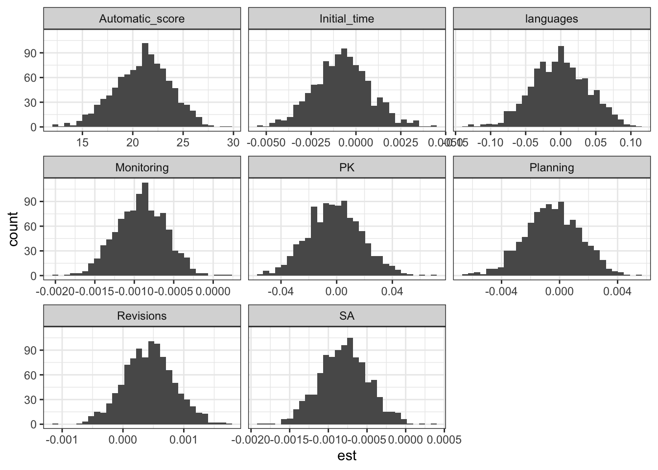
The distribution of regression coefficients across the 1,000 simulations is plotted below. As shown, the parameter estimates vary appropriately across replications:
`stat_bin()` using `bins = 30`. Pick better value `binwidth`.
A key point of concern in the original paper is the treatment of language as a predictor. Language was included as a single numeric variable, despite being a three-category nominal variable (English, German, Finnish). This is a clear misspecification: coding language as continuous imposes an arbitrary ordering and induces linear effects that have no meaningful interpretation. As a result, the claim that “Finnish led to improved automated scores” cannot be supported.
Even if we momentarily ignore the coding issue, one would expect no association between language and automated scoring if the scoring mechanism were unbiased across languages. Any non-zero effect would indicate a calibration issue.
More problematic is the paper’s claim of an indirect effect of language on human scores via the automated score. This is not supported by the model they presented:
no mediation pathway is explicitly specified;
there is no direct language → human path;
and conceptually, it is unclear how an automated scoring mechanism could mediate a causal relationship between language and human judgements.
In short, the model structure in the paper does not justify the inferential claims made about language, and the parameterisation prevents meaningful interpretation.
Conclusion
The simulations demonstrate that, when the model is specified as depicted in the paper, it produces a normal range of fit indices centred around RMSEA ≈ .07 and CFI ≈ .90, with substantial variation across replications. This is what we would expect from a model with seven degrees of freedom and no hidden parameters. In contrast, the published study reports nearly perfect fit (e.g., RMSEA ≈ 0, CFI = 1) based on a model with one degree of freedom. These results are incompatible. The only way their model could achieve the reported fit is if additional free parameters were estimated but not presented. Most plausibly, residual covariances or mean structure components. This renders the model almost saturated. In such a scenario, excellent fit is not evidence of a good model; it is an inevitability.
Beyond the fit issue, the treatment of language is especially problematic. The paper includes language as a single numeric predictor, despite the data involving three distinct linguistic groups. This coding error imposes an artificial ordering on categories (e.g., English < German < Finnish), generating regression effects that have no legitimate interpretation. Any claim that “Finnish students scored higher” or that “language predicted automated scores” is therefore unsupported. Even if the coding had been correct, a construct-relevant language effect would still be unexpected, as a fair scoring system should not advantage any language group.
This issue becomes even more concerning when the paper suggests an indirect effect of language on human scores viaautomated scoring. The model they present does not include the necessary structure for mediation, but more importantly, the claim is conceptually incoherent. Automated scoring cannot serve as a mediator between language and human judgement; any association is far more likely an artefact of measurement non-equivalence across languages, not a meaningful psychological mechanism. Treating measurement bias as a causal pathway fundamentally misrepresents what the model can show.
Taken together, the inconsistencies in reported fit, the incorrect handling of categorical predictors, and the conceptual leap from measurement artefact to psychological mediation raise substantial concerns about the validity of the study’s conclusions. Simulations using the reported summary statistics indicate that the theoretical model, when properly specified, does not support the strong claims made in the paper.