library(corrplot)
library(data.table)
library(flextable)
library(ggplot2)
library(haven)
library(lavaan)
library(mclust)
library(mirt)
library(psych)

scale_data <-
    read_sav("S DATA - Copy (2).sav") |>
as.data.table()This post seeks to explore Al-Qerem et al.’s (2026) validation of the Post-COVID-19 Symptom Scale (PCSS) for an Arabic population.
The PCSS is a 24-item measure capturing psychological, sensory, cognitive, and pain-related domains using an 11-point (0–10) severity scale. Original validation of this measure is attributed to Kuo et al. (2024). These authors found a five-factor model to fit the data. The latter is tenuous given the alternative fit measures (CFI = 0.922, TLI = 0.910, RMSEA = 0.073, and SRMR = 0.077); four freely correlated residuals were added to achieve this model fit. Without modifications, the model is a poor fit to the data (CFI = 0.873, TLI = 0.855, RMSEA = 0.093, and SRMR = 0.075). Notably, all four added residual correlations sit within rather than between factors. Items already grouped together needed extra covariance absorbed before the model would fit, which is itself a sign of redundant, overlapping content rather than five cleanly separable constructs.
The factors measured are as follows:
Life Threatening Concern
Cognitive Concern
Psychological and Non-Life Threatening Concern
Ache Concern
Sensory Concern
From a content perspective, Life Threatening Concern is measured by headache, vertigo, tachycardia, heart palpitation, difficulty breathing, and chest pain. The cardiac and respiratory items here are defensible groupings under a “life-threatening” label, but headache and vertigo sit awkwardly alongside them. Neither is typically life-threatening, and their inclusion looks more like a residual neurological/dizziness pairing than a genuine fit with the factor’s stated theme.
Cognitive Concern is measured by fatigue, brain fog, difficulty remembering, and difficulty concentrating. Kuo et al. note that fatigue stands out among these symptoms, implying a problematic structure; fatigue is not a cognitive symptom in any specific sense, and its presence here is explained post hoc rather than resolved.
Psychological and Non-Life Threatening Concern appears as an incoherent cluster of mental health concerns (e.g., depression, anxiety) and somatic concerns (e.g., dry mouth, hair loss, diarrhea, poor appetite). There is no obvious shared construct here beyond “didn’t fit anywhere else”.
Sensory Concern is worth flagging separately: it comprises only two items, anosmia and ageusia. A two-indicator factor is just-identified by construction, meaning its internal fit can’t be meaningfully tested, it’s structurally weak regardless of content coherence.
Taken together, the original PCSS factor structure was already fragile before any translation occurred: propped up by post hoc modification, built on at least two conceptually incoherent or structurally thin factors, and inheriting content groupings that the original authors themselves flagged as imperfect without resolving.
Al-Qerem et al.’s validation in an Arabic population found the five-factor model to have acceptable fit (CFI = 0.95, TLI = 0.95, SRMR = 0.02). Cronbach’s alpha values were at least 0.97. At face value, the scale appears good, with excellent reliability. However, these alpha values suggest apparent redundancy in item content rather than genuine subscale precision. Values this high, this uniformly, across every factor are more consistent with items that are near-interchangeable than with five distinct, well-measured constructs. As the data for this study is openly accessible, we can re-evaluate the scale.
The following approach will be taken:
Item response distributions and correlations will be explored to identify item ceiling/floor effects and item redundancies.
An exploratory factor analysis (EFA) will be run to understand whether the original five-factor model holds up using the Al-Qerem et al. data. Only a confirmatory factor analysis (CFA) was run in the original validation, as opposed to exploring model variations.
An item response model is run to explore how the 24 items of the PCSS function.
A final mixture model of total scores is run to understand how individuals complete the PCSS scale.
Response Distributions and Correlations
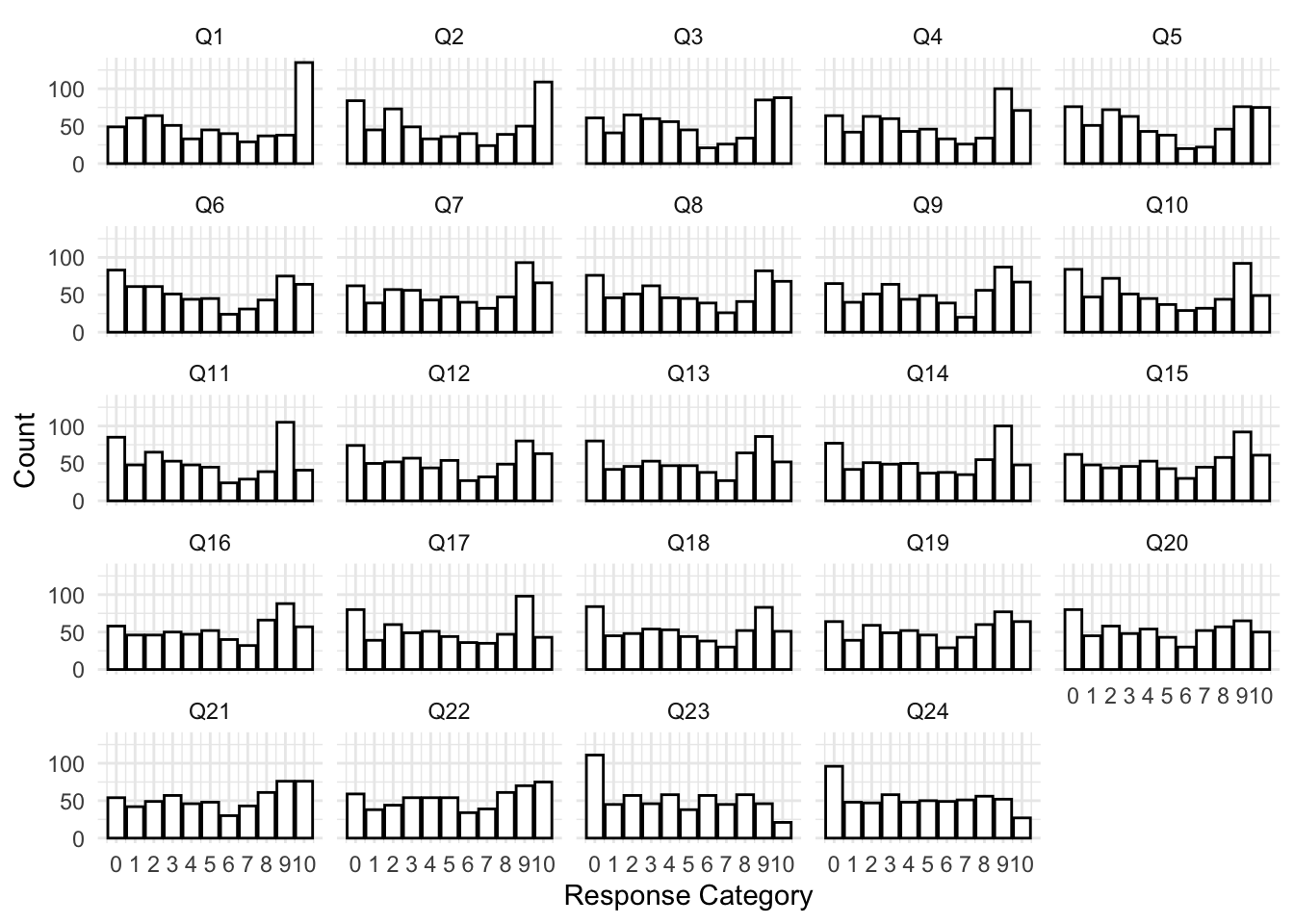
Response distributions across the 24 PCSS items are predominantly bimodal, with elevated counts at the scale extremes (0 and 10) and a relative depletion of the middle response categories. This pattern suggests respondents are using the 0–10 scale in a largely polarised way, endorsing either minimal or severe symptom levels, rather than making fine-grained distinctions across the full range, consistent with the category functioning observed later in the IRT (item response theory) analysis. A smaller subset of items (Q18, Q23, and Q24) show a clear floor effect, with responses declining from 0 and no corresponding peak at the upper end.
scale_data |>
    melt(
        id.vars = "ID",
        measure.vars = patterns("^Q"),
        variable.name = "item",
        value.name = "response"
    ) |>
    ggplot(aes(x = response)) +
    stat_count(
        colour = "black",
        fill = "white"
    ) +
    facet_wrap(~item) +
    scale_x_continuous(breaks = 0:10*1) +
    theme_minimal() +
    labs(
        x = "Response Category",
        y = "Count"
    )
Correlations between items are uniformly high (median = 0.83), with no visible block structure corresponding to the five hypothesised factors. This pattern is consistent with a dominanant general factor rather than five individual dimensions.
cor(scale_data[, .SD, .SDcols = patterns("^Q")]) |>
    corrplot(method = "number", type = "lower")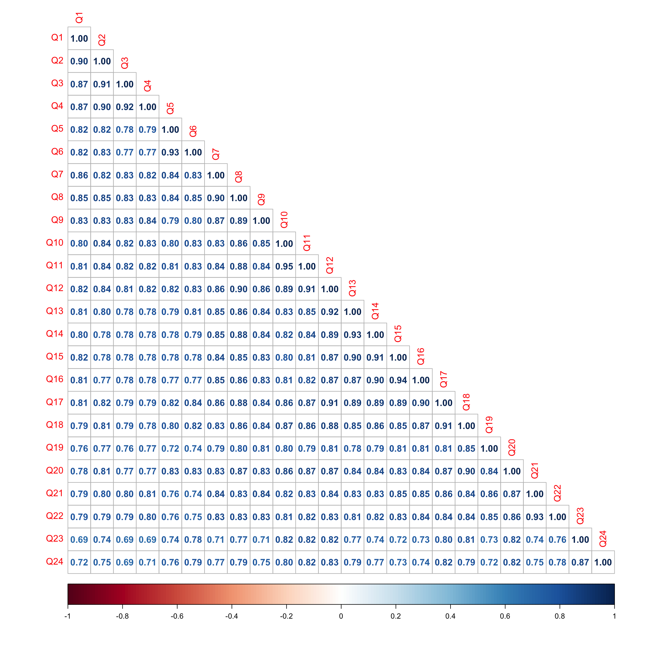
Exploratory Factor Analysis
The PCSS is purported to measure five concern factors. Here we run a parallel analysis of the scale data. Contrary to Kuo et al. and Al-Qerem et al., we find that a three factor solution is considered optimal.
fa.parallel(scale_data[, .SD, .SDcols = patterns("^Q")])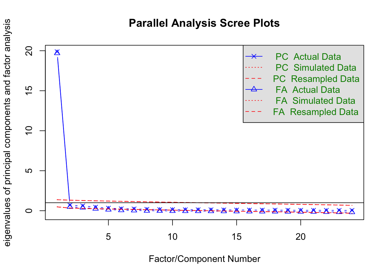
Parallel analysis suggests that the number of factors = 3 and the number of components = 1 Three-Factor Solution
If we run the EFA with three factors, the obtained fit is poor and notably worse than the fit reported for the original five-factor model, despite being the statistically recommended solution.
efa_mod <-
  efa(scale_data[, .SD, .SDcols = patterns("^Q")], nfactors = 3, ordered = T)

fitmeasures(
  efa_mod,
  fit.measures = c(
    "chisq.scaled", "df.scaled", "pvalue.scaled", "cfi.robust", "rmsea.robust"
    )
  ) |>
  as.data.table(keep.rownames = T) |>
  flextable() |>
  colformat_double(digits = 2) |>
  align_nottext_col(align = "center") |>
  set_header_labels(values = c("Fit Measure", "Factors = 3")) |>
  autofit()
Fit Measure | Factors = 3 |
|---|---|
chisq.scaled | 4,267.26 |
df.scaled | 207.00 |
pvalue.scaled | 0.00 |
cfi.robust | 0.84 |
rmsea.robust | 0.19 |
Loadings from the three-factor solution show clear problems.
Factor 1 captures the cognitive/psychological items, with the two sensory items (Q5, Q6) cross-loading here more strongly than on their own factor.
Factor 2 emerges as a weak residual sensory factor, with Q5 and Q6 as its only items and at loadings (0.35–0.39) considerably lower than their loadings on Factor 1. This suggests sensory content is not cleanly separable from the cognitive cluster in this data.
Factor 3 absorbs the remaining items but with markedly uneven loading strength: the cardiac/life-threatening items (Q7–Q11) load weakly and diffusely (0.41–0.58), while the ache items (Q13–Q16) produce clear Heywood cases, with standardized loadings of 1.18 to 1.28.
This is a sign the three-factor solution is not well identified for this item set, independent of its already-poor fit indices.
efa_loadings <-
  efa_mod$loadings |>
  as.data.table(keep.rownames = T)

cols <- c("f1", "f2", "f3")
efa_loadings[, (cols) := lapply(.SD, function (x) fifelse(x < 0.30, NA, x)), .SDcols = cols]

efa_loadings |>
  flextable() |>
  colformat_double(digits = 2) |>
  align_nottext_col(align = "center") |>
  set_header_labels(values = c("Items", "Factor 1", "Factor 2", "Factor 3")) |>
  autofit()
Items | Factor 1 | Factor 2 | Factor 3 |
|---|---|---|---|
Q1 | 0.77 | ||
Q2 | 0.91 | ||
Q3 | 0.98 | ||
Q4 | 0.93 | ||
Q5 | 0.88 | 0.35 | |
Q6 | 0.85 | 0.39 | |
Q7 | 0.41 | 0.54 | |
Q8 | 0.38 | 0.58 | |
Q9 | 0.38 | 0.57 | |
Q10 | 0.45 | 0.49 | |
Q11 | 0.42 | 0.52 | |
Q12 | 0.81 | ||
Q13 | 1.18 | ||
Q14 | 1.28 | ||
Q15 | 1.25 | ||
Q16 | 1.24 | ||
Q17 | 0.93 | ||
Q18 | 0.91 | ||
Q19 | 0.85 | ||
Q20 | 0.81 | ||
Q21 | 0.96 | ||
Q22 | 0.96 | ||
Q23 | 0.82 | ||
Q24 | 0.81 |
Inter-factor correlations confirm this picture: Factor 1 and Factor 3 correlate at 0.91, sharing roughly 83% of their variance, which is well beyond any reasonable threshold for claiming the two are empirically distinct constructs. Factor 2 (sensory) is essentially uncorrelated with the other two.
lavInspect(efa_mod$nf3, what = "std.lv")$psi f1 f2 f3
f1 1.000
f2 0.079 1.000
f3 0.914 0.160 1.000Taken together, the loadings, fit indices, and inter-factor correlations all point toward a single dominant factor, with sensory items forming, at most, a weak secondary cluster.
One-Factor Solution
A unidimensional model is tested as the simplest possible structure. Its fit is worse than the three-factor solution above (CFI = 0.79, RMSEA = 0.20 vs CFI = 0.84, RMSEA = 0.19), despite producing the cleanest loading pattern of any model tested.
efa_mod <-
  efa(scale_data[, .SD, .SDcols = patterns("^Q")], nfactors = 1, ordered = T)

fitmeasures(
  efa_mod,
  fit.measures = c(
    "chisq.scaled", "df.scaled", "pvalue.scaled", "cfi.robust", "rmsea.robust"
  )
) |>
  as.data.table(keep.rownames = T) |>
  flextable() |>
  colformat_double(digits = 2) |>
  align_nottext_col(align = "center") |>
  set_header_labels(values = c("Fit Measure", "Factors = 1")) |>
  autofit()
Fit Measure | Factors = 1 |
|---|---|
chisq.scaled | 5,602.94 |
df.scaled | 252.00 |
pvalue.scaled | 0.00 |
cfi.robust | 0.79 |
rmsea.robust | 0.20 |
No Heywood cases are present in the one-factor solution, and all items load cleanly and uniformly, in a narrow band from 0.87 to 0.95.
efa_loadings <-
  efa_mod$loadings |>
  as.data.table(keep.rownames = T)

cols <- c("f1", "f2", "f3")
efa_loadings[, f1 := fifelse(f1 < 0.30, NA, f1)]

efa_loadings |>
  flextable() |>
  colformat_double(digits = 2) |>
  align_nottext_col(align = "center") |>
  set_header_labels(values = c("Items", "Factor 1")) |>
  autofit()
Items | Factor 1 |
|---|---|
Q1 | 0.91 |
Q2 | 0.92 |
Q3 | 0.92 |
Q4 | 0.92 |
Q5 | 0.93 |
Q6 | 0.93 |
Q7 | 0.92 |
Q8 | 0.94 |
Q9 | 0.91 |
Q10 | 0.94 |
Q11 | 0.95 |
Q12 | 0.95 |
Q13 | 0.95 |
Q14 | 0.95 |
Q15 | 0.94 |
Q16 | 0.94 |
Q17 | 0.95 |
Q18 | 0.94 |
Q19 | 0.87 |
Q20 | 0.93 |
Q21 | 0.93 |
Q22 | 0.93 |
Q23 | 0.87 |
Q24 | 0.87 |
Across all three models tested: five-factor (Al-Qerem et al.’s reported structure), three-factor (parallel-analysis-recommended), and one-factor, no solution is unambiguously well-supported. The five-factor model achieves the best conventional fit statistics, but only by allowing a highly parameterised, freely correlated structure to absorb what these analyses suggest is fundamentally a single dominant dimension.
Item Response Theory
We can dig further into the scale through the use of IRT. Below we apply a graded response model (GRM) to the 24 items, assuming a unidimensional model – the structure supported by the EFA above.
graded_mod <-
  mirt(
    scale_data[, .SD, .SDcols = patterns("^Q")],
    model = 1,
    itemtype = "graded")
As with the EFA fit, the graded model does not fit the data well (RMSEA = 0.11). A note: we also received a warning that the null-model chi-squared was smaller than the fitted model.
M2(graded_mod) |>
  flextable() |>
  colformat_double(digits = 2)
Warning: Null model chi-squared value smaller than fitted modelM2 | df | p | RMSEA | RMSEA_5 | RMSEA_95 | SRMSR |
|---|---|---|---|---|---|---|
294.78 | 36 | 0.00 | 0.11 | 0.10 | 0.12 | 0.04 |
If we look at item probability functions, we clearly see the issue with this scale: disordered thresholds. Several adjacent response categories never become the most probable response at any point along the latent trait — there is no position on the severity continuum where, for example, a respondent is genuinely more likely to select “4” than either “3” or “5.” Small, often negligible increments in the underlying latent severity are being mapped onto large, discrete jumps in observed response category, with the middle of the scale collapsing into functionally indistinguishable options.
plot(graded_mod, type = "trace", which.item = 5:6)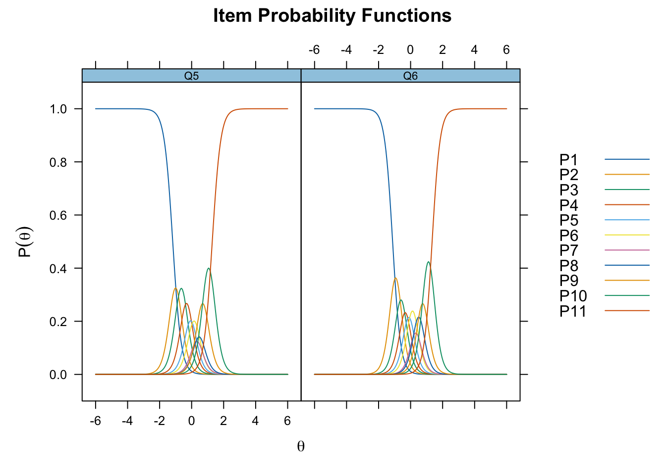
The same pattern holds for item 24. The limitations of an 11-point severity scale are clearly showcased here: respondents are functionally choosing between a small number of meaningfully distinct severity levels, not 11.
plot(graded_mod, type = "trace", which.item = 24)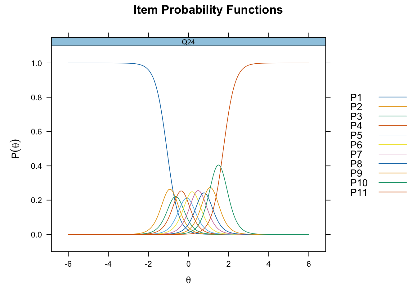
Collapsed Response Categories
As a final step, we can collapse response categories:
0: Absent
1-3: Mild
4-6: Moderate
7-9: Severe
10: Extreme
cols <- grep("^Q", names(scale_data), perl = T, value = T)
scale_data[, (cols) := lapply(.SD, function (x) {
  fcase(
    x == 0, 0,
    x %in% c(1, 2, 3), 1,
    x %in% c(4, 5, 6), 2,
    x %in% c(7, 8, 9), 3,
    x == 10, 4
  )
}), .SDcols = cols]
Again, we re-run the graded response model with an assumed single factor.
graded_mod <-
  mirt(
    scale_data[, .SD, .SDcols = patterns("^Q")],
    model = 1,
    itemtype = "graded")
With collapsed categories, the M2 routine runs without the null-model warning seen previously, consistent with a better-identified model. Fit improves on the relative indices (CFI = 0.91, TLI = 0.90), crossing the conventional acceptability threshold. RMSEA remains unchanged at 0.11, however, still outside the conventional good-fit range. This pattern suggests collapsing categories resolves the scale-format problem (disordered thresholds) without fully resolving the broader item redundancy and dimensionality issues documented throughout this analysis; the two are related but distinct problems, and category collapsing only addresses the former.
M2(graded_mod) |>
  flextable() |>
  colformat_double(digits = 2)
M2 | df | p | RMSEA | RMSEA_5 | RMSEA_95 | SRMSR | TLI | CFI |
|---|---|---|---|---|---|---|---|---|
1,448.66 | 180 | 0.00 | 0.11 | 0.10 | 0.12 | 0.04 | 0.90 | 0.91 |
The response curves bear this out. Threshold disordering is no longer apparent: each of the five collapsed categories now occupies a distinct region of the latent trait where it is the most probable response, rather than the compressed, overlapping pattern seen under the original 11-point scale.
plot(graded_mod, type = "trace")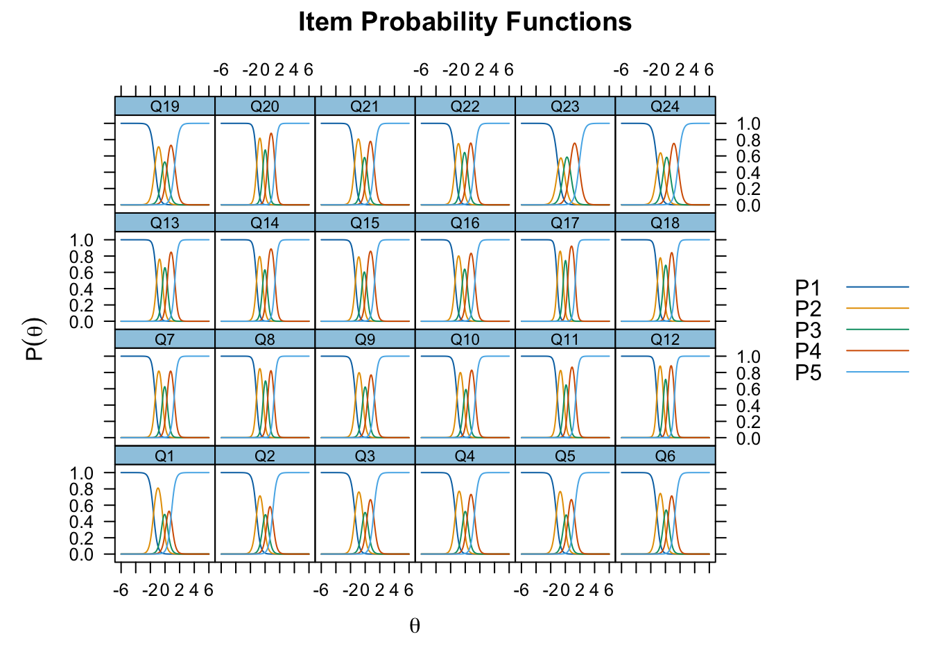
Summary
Al-Qerem et al. and Kuo et al. claim that the PCSS measures five factors with excellent fit and reliability. This is what was tested here using the open data of Al-Qerem et al. The short answer: it doesn’t hold up.
We adopted a systematic approach in this post, starting from descriptive statistics of the scale (distributions and correlations), through exploring various factor solutions, culminating in an exploration of item functioning. Response distributions were predominantly bimodal, with respondents clustering at the scale extremes rather than using the full 0–10 range, and inter-item correlations were uniformly high with no block structure corresponding to five factors. Parallel analysis recommended three factors, agreeing with neither Kuo et al. nor Al-Qerem et al., but the three-factor solution produced Heywood cases and fit worse than even a single factor. The one-factor solution, by contrast, gave clean, uniform loadings across all 24 items, though its fit was also poor by conventional SEM standards.
A graded response model confirmed the same picture from an entirely different modelling framework: poor fit, and disordered category thresholds across most items, with several middle response categories never the most probable response at any point along the latent trait. This is the mechanism underlying everything above. The 11-point severity scale invites a polarised absent/severe response style rather than genuine graded discrimination, which inflates inter-item correlations, produces an artificially dominant general factor, and is almost certainly what allowed a five-factor CFA, tested with no model comparison or alternative structures, to report excellent fit on data that isn’t five-dimensional at all. Collapsing the scale to five broader categories partially resolved the threshold disordering and improved relative fit indices, though RMSEA remained elevated, indicating the category-collapsing fixes the scale-format problem without fully resolving the underlying item redundancy.
None of this means the PCSS-Ar is unusable. The items still capture meaningful post-COVID symptom content, and the translation and DIF work in Al-Qerem et al. appear sound. What doesn’t survive is the five-factor structure and any scoring or interpretation at the subscale level. A unidimensional total score, ideally collected on a shorter, properly functioning response scale, is what this data actually supports.