Alex Wainwright - Fixing What’s Broken: Refining a Social Media Use Scale Through Rigorous Analysis

Social media platforms have become integral to daily communication and self-expression, yet measuring how people actually use these platforms remains challenging. While objective metrics like screen time provide some insight, they miss the nuanced behaviors that define social media engagement, from carefully curating posts to mindlessly scrolling through feeds.

The Social Media Use (SMU) scale was developed to capture these behavioral patterns through a 17-item measure of image management, social comparison, and content consumption. However, this streamlined version emerged from a larger 31-item pool, and the reduction process may have obscured important distinctions in how people engage with social platforms.

This analysis revisits the original 31-item scale to examine whether the current factor structure adequately captures the complexity of social media behavior, with particular attention to response patterns and item performance that may have been overlooked in previous validation work.

# Library ---------------------
library(data.table)
library(flextable)
library(ggplot2)
library(lavaan)
library(readxl)

# Read Study Data -------------
study_two_data <- 
  read_xlsx("Study 2 Data.xlsx") |>
  as.data.table()

study_three_data <- 
  read_xlsx("Study 3 Data.xlsx") |>
  as.data.table()

item_wording <-
  read.csv("study2_item_wording_only.csv")

The original and current SMU scales ask respondents to indicate how frequently they engaged in specific activities over the previous seven days across any combination of platforms, including Facebook, Instagram, Twitter, Snapchat, Reddit, Tumblr, and LinkedIn. Each item uses a nine-point Likert scale from 1 (Never) to 9 (Hourly or more).

The complete 31-item pool, along with the theoretical factors each item was designed to measure, is presented below:

Item #	Item	Model 1
1	Made/shared a post or story about fundraising or benefits	Voicing
2	Made/shared a post or story advertising events or meetups	Voicing
3	Made/shared a post or story about something negative that was NOT personally about me	Voicing
4	Signed a petition or donated money to a cause	Voicing
5	Commented unsupportively or disliked/“reacted” unsupportively on other’s post(s)	Voicing
6	Made/shared a post or story about something positive that was NOT personally about me	Voicing
7	Sought out the profile of someone I dislike (“hate stalked”)	Voicing
8	Made/shared a post or story about something negative that was personally about me	Voicing
9	Made/shared a post or story about something positive that was personally about me	Voicing
10	Sought out entertaining content other than videos or memes	Content seeking
11	Sought out content that I morally or ethically agreed with	Content seeking
12	Watched videos that were NOT memes, news content, or how-tos/recipes	Content seeking
13	Read, watched, or caught up on news or current events	Content seeking
14	Sought out content that I morally or ethically disagreed with	Content seeking
15	Navigated to interest groups’ feeds (e.g., searching for hashtags, visiting a subreddit)	Content seeking
16	Viewed events in my area	Content seeking
17	Looked at others’ stories	Browsing
18	Scrolled aimlessly through my feed(s)	Browsing
19	Read through my notifications	Browsing
20	Navigated to others’ profiles in my social network (e.g., friends or friends of friends)	Browsing
21	Looked at or watched memes	Browsing
22	Looked at or watched videos such as how-tos/recipes, and DIY projects	Browsing
23	Read comments to my own content	Image Managing
24	Looked at how many people liked, commented on, shared my content, or followed/friended me	Image Managing
25	Commented supportively or liked/“reacted” supportively on other’s post(s)	Image Managing
26	Compared my body or appearance to others’	Image Managing
27	Edited and/or deleted my own social media content	Image Managing
28	Compared my life or experiences to others’	Image Managing
29	Reminisced about the past	Image Managing
30	Played with photo filtering/photo editing	Image Managing
31	Navigated to others’ pages who I do not know (e.g., influencers or other famous people)	Image Managing

Exploring the Data

Initial examination of the response distributions across all 31 items reveals significant floor effects in the data. Figure 1 displays the frequency distributions for each item, showing that many behaviors were rarely endorsed by participants.

smu_study_two <- 
  study_two_data[, .SD, .SDcols = patterns("^Act_")]

smu_study_two[, index := .I]

smu_study_two_long <-
  smu_study_two |>
  melt(id.vars = "index",
       variable.name = "item",
       value.name = "response")

smu_study_two_long[, .N, by = .(item, response)] |>
  ggplot(aes(x = response, y = N)) +
  geom_col() +
  facet_wrap(~item) +
  theme_bw() +
  labs(x = "Response Option") +
  scale_x_continuous(breaks = seq(1, 9, 1))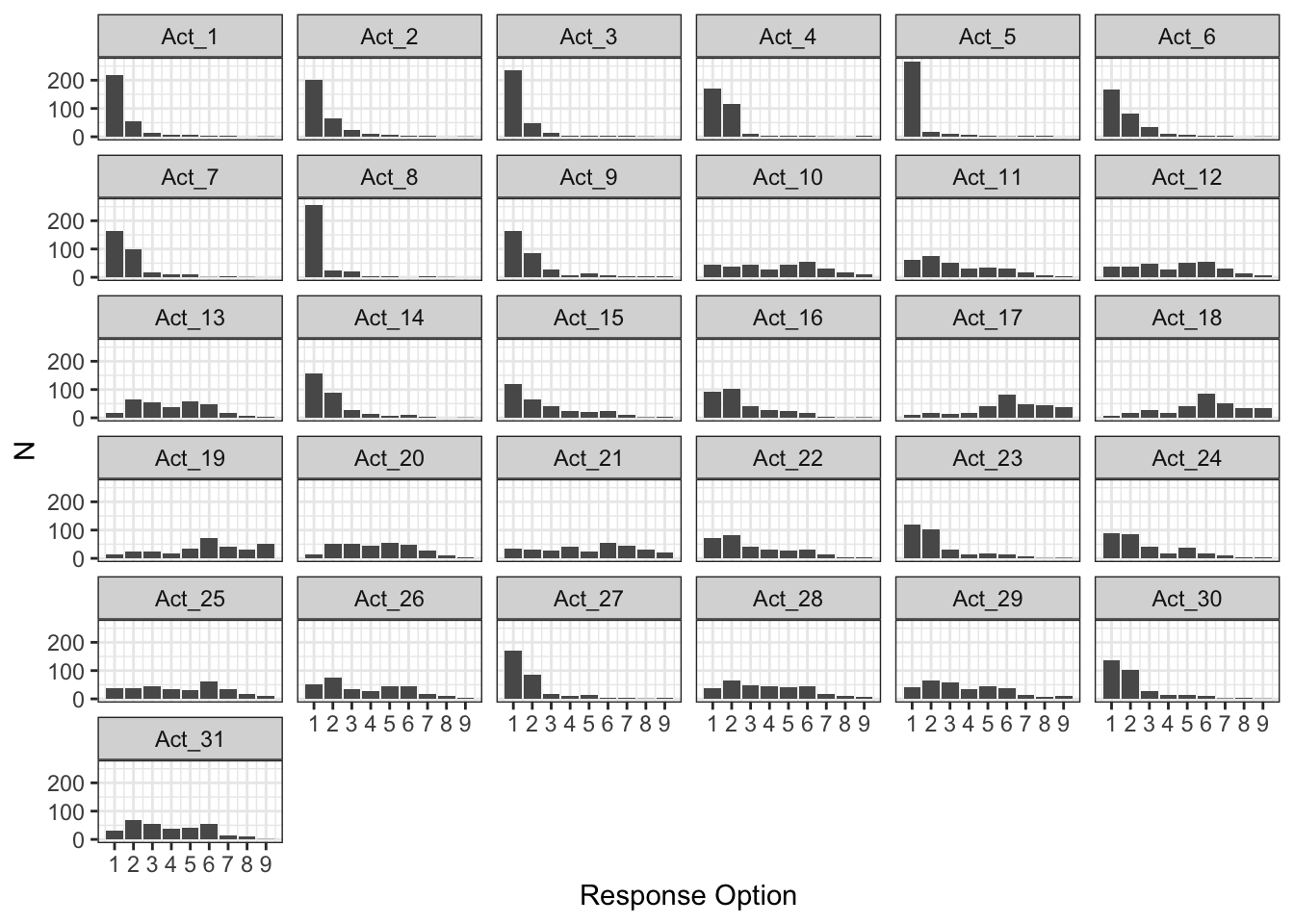

Figure 1: Response distributions for the 31 SMU scale items

To quantify these floor effects, Table 1 presents the proportion of respondents who selected “Never” (response option 1) for each item. Using a 50% threshold as indicative of problematic floor effects, 11 items (35.48% ) demonstrate concerning response patterns.

item_response_proportion <-
  smu_study_two[, .(item = names(.SD),
                    proportion = apply(.SD, 2, function(x)
                      round(mean(x == 1, na.rm = T) * 100, 2))),
                .SDcols = patterns("^Act_")][order(proportion, decreasing = T)][proportion >= 50] 

item_response_proportion |>
  as_flextable(
    max_row = 31, 
    show_coltype = F) |>
  set_header_labels(values = c("Item", "%"))

Table 1: Items with floor effects (≥50% “Never” responses)
Item	%
Act_5	85.8
Act_8	82.6
Act_3	75.9
Act_1	70.4
Act_2	64.3
Act_4	55.3
Act_27	55.3
Act_6	53.4
Act_7	53.0
Act_9	52.7
Act_14	50.5
n: 11

These 11 problematic items fall into several behavioral categories:

Antisocial/Negative Behaviors:

Commented unsupportively or disliked posts (Act_5: 85.8%)
Sought out profiles of disliked individuals (Act_7: 53.0%)

Negative Content Sharing:

Posted negative content about oneself (Act_8: 82.6%)
Posted negative content about others (Act_3: 75.9%)

Advocacy/Cause-Related Activities:

Posted about fundraising or benefits (Act_1: 70.4%)
Posted about events or meetups (Act_2: 64.3%)
Signed petitions or donated to causes (Act_4: 55.3%)

Deliberate Content Curation:

Edited or deleted own content (Act_27: 55.3%)
Sought out disagreeable content (Act_14: 50.5%)

These floor effects are understandable given the behaviors measured and the seven-day timeframe. Antisocial behaviors like unsupportive commenting represent socially undesirable actions that most users avoid. Similarly, sharing negative personal content contradicts typical social media norms of presenting an idealised self. Advocacy-related activities, while positive, may occur sporadically rather than within any given week. The brief timeframe likely exacerbates these patterns, behaviors that might occur monthly or yearly appear as “never” when assessed over seven days.

Initial Model Fitting

Testing the hypothesised four-factor structure with all 31 items immediately revealed computation problems. The confirmatory factor analysis failed to converge properly, generating a warning about matrix singularity:

four_factor_model <- "
  voicing =~ Act_1 + Act_2 + Act_3 + Act_4 + Act_5 + Act_6 + Act_7 + Act_8 + Act_9
  content_seeking =~ Act_10 + Act_11 + Act_12 + Act_13 + Act_14 + Act_15 + Act_16
  browsing =~ Act_17 + Act_18 + Act_19 + Act_20 + Act_21 + Act_22
  image_managing =~ Act_23 + Act_24 + Act_25 + Act_26 + Act_27 + Act_28 + Act_29 + Act_30 + Act_31
"

tryCatch(
  cfa(four_factor_model,
      data = smu_study_two,
      ordered = T,
      estimator = "WLSMV"),
  warning = function (x)
    paste0(x$message)
)

[1] "lavaan WARNING:\n    The variance-covariance matrix of the estimated parameters (vcov)\n    does not appear to be positive definite! The smallest eigenvalue\n    (= -8.463758e-17) is smaller than zero. This may be a symptom that\n    the model is not identified."

This computational failure likely stems from the severe floor effects identified earlier. When most respondents respond “Never” to certain items, the resulting correlation matrices can become unstable, leading to estimation problems in factor analysis.

Addressing the Floor Effects

Two potential solutions emerged:

Collapse response scales - Convert the 9-point scales to binary (Never vs. Any engagement) for all items
Remove problematic items - Drop the 11 items showing severe floor effects

Approach 1: Item Removal

Initially, I attempted the second approach, removing all 11 items with floor effects above 50%. However, even with the reduced 20-item set, exploratory factor analysis continued to produce the same matrix singularity warnings.

items_to_drop <-
  item_response_proportion[, item]
smu_study_two[, (items_to_drop) := NULL]

tryCatch(
  efa(data = smu_study_two[, .SD, .SDcols = patterns("^Act_")],
    ordered = T,
    nfactors = 1:4, 
    rotation = "geomin"),
  warning = function (x)
    paste0(x$message)
)

[1] "lavaan WARNING:\n    The variance-covariance matrix of the estimated parameters (vcov)\n    does not appear to be positive definite! The smallest eigenvalue\n    (= -4.788696e-17) is smaller than zero. This may be a symptom that\n    the model is not identified."

The persistence of computational problems suggested that floor effects were more pervasive than initially apparent, or that removing these items created other structural issues in the data. This led to reconsidering the first approach: collapsing the response scale entirely.

Binary Scale Transformation

Given the persistent computational issues, I implemented a more extreme solution: collapsing all 31 items from the original 9-point scale to a binary format (0 = Never, 1 = Any engagement within 7 days). While this approach sacrifices information about frequency gradations, it directly addresses the floor effect problems and aligns with a key research question: did respondents engage in these behaviors at all during the past week?

smu_study_two <- 
  study_two_data[, .SD, .SDcols = patterns("^Act_")]

smu_study_two <-
  smu_study_two[, apply(.SD, 2, function (x) fifelse(x > 1, 1, 0)), .SDcols = patterns("^Act_")] |>
  as.data.table()

Model Convergence and Fit

The binary transformation resolved the computation issues entirely. The four factor confirmatory factor analysis converged without warnings and produced interpretable results:

four_factor_model <- "
  voicing =~ Act_1 + Act_2 + Act_3 + Act_4 + Act_5 + Act_6 + Act_7 + Act_8 + Act_9
  content_seeking =~ Act_10 + Act_11 + Act_12 + Act_13 + Act_14 + Act_15 + Act_16
  browsing =~ Act_17 + Act_18 + Act_19 + Act_20 + Act_21 + Act_22
  image_managing =~ Act_23 + Act_24 + Act_25 + Act_26 + Act_27 + Act_28 + Act_29 + Act_30 + Act_31
"

cfa_model <- tryCatch(
  cfa(
    four_factor_model,
    data = smu_study_two,
    ordered = T,
    estimator = "WLSMV"
  ),
  warning = function (x)
    paste0(x$message)
)

fitmeasures(cfa_model, fit.measures = c("chisq.scaled", "df.scaled", "pvalue.scaled", "cfi.scaled", "tli.scaled", "rmsea.scaled")) |>
  as.data.table(keep.rownames = T) |>
  _[, V1 := c(
    "χ² (scaled)",
    "df",
    "p-value",
    "CFI",
    "TLI",
    "RMSEA"
  )] |>
  as_flextable(show_coltype = F) |>
  colformat_double(digits = 2) |>
  set_header_labels(
    values = c("Fit Index", "Value")
  )

Table 2: Model Fit Indices for Four-Factor Binary Model
Fit Index	Value
χ² (scaled)	621.32
df	428.00
p-value	0.00
CFI	0.94
TLI	0.94
RMSEA	0.04
n: 6

While the significant chi-square indicates exact model-data misfit, the relative fit indices suggest reasonable approximation. Both CFI and TLI exceed 0.90, and RMSEA falls within acceptable bounds (< 0.06).

Factor Loadings

Factor loadings ranged from 0.47 to 0.87 across all items (Table 3), indicating moderate to strong relationships between items and their intended factors. Using a conventional threshold of λ ≥ 0.70 for strong loadings, 12 items showed weaker associations with their factors.

 cfa_model_loadings <- 
   inspect(cfa_model, what = "std")$lambda |>
   as.data.table(keep.rownames = T)
 
 cfa_model_loadings[, c("voicing", "content_seeking", "browsing", "image_managing") := lapply(.SD, function (x) fifelse(x == 0, NA_integer_, x)), .SDcols = c("voicing", "content_seeking", "browsing", "image_managing")] |>
   as_flextable(max_row = 31,
                show_coltype = F) |>
   colformat_double(digits = 2)

Table 3: Standardised Factor Loadings
rn	voicing	content_seeking	browsing	image_managing
Act_1	0.78
Act_2	0.71
Act_3	0.82
Act_4	0.68
Act_5	0.60
Act_6	0.80
Act_7	0.61
Act_8	0.81
Act_9	0.81
Act_10		0.60
Act_11		0.81
Act_12		0.53
Act_13		0.47
Act_14		0.75
Act_15		0.59
Act_16		0.72
Act_17			0.87
Act_18			0.85
Act_19			0.68
Act_20			0.82
Act_21			0.54
Act_22			0.61
Act_23				0.80
Act_24				0.83
Act_25				0.82
Act_26				0.55
Act_27				0.73
Act_28				0.68
Act_29				0.71
Act_30				0.83
Act_31				0.74
n: 31

Item Difficulty and Threshold Analysis

The threshold parameters reveal interesting patterns about item “difficulty” in the binary context (Table 4). Voicing items generally showed positive thresholds (particularly Act_5: 1.07, Act_8: 0.94), indicating these behaviours require higher levels of the underlying trait to endorse. Conversely, most browsing and content-seeking items showed negative thresholds, suggesting these are “easier” behaviors that most people engage in regardless of their trait levels.

inspect(cfa_model, what = "std")$tau |>
  as.data.table(keep.rownames = T) |>
  as_flextable(max_row = 31,
               show_coltype = F) |>
  colformat_double(digits = 2) |>
  set_header_labels(
    values = c("Item", "Threshold")
  )

Table 4: Item Thresholds
Item	Threshold
Act_1\|t1	0.53
Act_2\|t1	0.36
Act_3\|t1	0.70
Act_4\|t1	0.13
Act_5\|t1	1.07
Act_6\|t1	0.08
Act_7\|t1	0.07
Act_8\|t1	0.94
Act_9\|t1	0.06
Act_10\|t1	-1.07
Act_11\|t1	-0.85
Act_12\|t1	-1.16
Act_13\|t1	-1.54
Act_14\|t1	0.01
Act_15\|t1	-0.30
Act_16\|t1	-0.53
Act_17\|t1	-1.85
Act_18\|t1	-1.95
Act_19\|t1	-1.69
Act_20\|t1	-1.66
Act_21\|t1	-1.21
Act_22\|t1	-0.72
Act_23\|t1	-0.29
Act_24\|t1	-0.58
Act_25\|t1	-1.16
Act_26\|t1	-0.96
Act_27\|t1	0.13
Act_28\|t1	-1.19
Act_29\|t1	-1.12
Act_30\|t1	-0.15
Act_31\|t1	-1.28
n: 31

Local Fit Assessment

Examination of standardised residuals identified items contributing most to model misfit (Table 5). Fourteen items showed mean absolute residuals ≥ 0.10, with Act_18 (doomscrolling: 0.138) and Act_31 (viewing unknown profiles: 0.131) showing the largest discrepancies between observed and model-implied correlations.

This pattern of misfit, combined with loading strength and conceptual considerations, informed the subsequent scale refinement process.

apply(residuals(cfa_model)$cov, 1, function (x) mean(abs(x))) |>
  as.data.table(keep.rownames = T) |>
  _[V2 >= .10] |>
  _[order(-V2)] |>
  as_flextable(max_row = 31,
               show_coltype = F) |>
  colformat_double(digits = 3) |>
  set_header_labels(
    values = c("Item", "Mean Absolute Residual")
  )

Table 5: Mean Absolute Residuals
Item	Mean Absolute Residual
Act_18	0.138
Act_31	0.131
Act_5	0.128
Act_17	0.124
Act_29	0.123
Act_13	0.122
Act_19	0.121
Act_6	0.120
Act_7	0.119
Act_21	0.116
Act_9	0.113
Act_28	0.112
Act_27	0.111
Act_26	0.106
n: 14

Refining the Scale

The following items were identified for removal based on multiple criteria:

Item #	Wording	Issues
5	Commented unsupportively or disliked/“reacted”unsupportively	High Threshold (1.07), low loading (0.60), high mean absolute residual (0.128), conceptually questionable
7	Sought out the profile of someone I dislike (“hate stalked”)	Low loading (0.61), high residual (0.119), possibly socially undesirable
12	Watched videos that were NOT memes, news content, or how-tos/recipes	Low loading (0.53), may be conceptually vague
13	Read, watched, or caught up on news or current events	Low loading (0.47), high residual (0.122), conceptual mismatch with digital leisure/social use
15	Navigated to interest groups’ feeds (e.g., hashtags, subreddits)	Low loading (0.59), potentially too specific or blurred with browsing
21	Looked at or watched memes	Low loading (0.54), high residual (0.116), conceptually too general
26	Compared my body or appearance to others	Low loading (0.55), high residual (0.106), conceptually crosses into self-esteem/psych distress
28	Compared my life or experiences to others	Loading 0.68, residual 0.112 — conceptually similar to #26, may be duplicative/redundant

smu_study_two[, c("Act_5", "Act_7", "Act_12", "Act_13", "Act_15", "Act_21", "Act_26", "Act_28") := NULL]

four_factor_model <- "
  voicing =~ Act_1 + Act_2 + Act_3 + Act_4 + Act_6 + Act_8 + Act_9
  content_seeking =~ Act_10 + Act_11 + Act_14 + Act_16
  browsing =~ Act_17 + Act_18 + Act_19 + Act_20 + Act_22
  image_managing =~ Act_23 + Act_24 + Act_25 + Act_27 + Act_29 + Act_30 + Act_31
"

cfa_model <- tryCatch(
  cfa(
    four_factor_model,
    data = smu_study_two,
    ordered = T,
    estimator = "WLSMV"
  ),
  warning = function (x)
    paste0(x$message)
)

Revised Four-Factor Model

After removing the eight problematic items, the four-factor model was retested using the remaining 23-items.

Model Fit Results

The 23 item confirmatory factor analysis successfully converged with improved global fit (Table 6), although the Chi-Square test still suggests rejection of the exact model fit.

fitmeasures(cfa_model, fit.measures = c("chisq.scaled", "df.scaled", "pvalue.scaled", "cfi.scaled", "tli.scaled", "rmsea.scaled")) |>
  as.data.table(keep.rownames = T) |>
  _[, V1 := c(
    "χ² (scaled)",
    "df",
    "p-value",
    "CFI",
    "TLI",
    "RMSEA"
  )] |>
  as_flextable(show_coltype = F) |>
  colformat_double(digits = 2) |>
  set_header_labels(
    values = c("Fit Index", "Value")
  )

Table 6: Model Fit Indices for Four-Factor Binary Model using 23-Item Scale
Fit Index	Value
χ² (scaled)	324.89
df	224.00
p-value	0.00
CFI	0.97
TLI	0.96
RMSEA	0.04
n: 6

The CFI and TLI values above 0.95 and RMSEA below 0.05 indicate acceptable to good model fit despite the significant chi-square value.

Factor Loadings

All retained items demongrate moderate to strong factor loadings (Table 7), with the lowest being Act_22 (λ = 0.56).

 cfa_model_loadings <- 
   inspect(cfa_model, what = "std")$lambda |>
   as.data.table(keep.rownames = T)
 
 cfa_model_loadings[, c("voicing", "content_seeking", "browsing", "image_managing") := lapply(.SD, function (x) fifelse(x == 0, NA_integer_, x)), .SDcols = c("voicing", "content_seeking", "browsing", "image_managing")] |>
   as_flextable(max_row = 31,
                show_coltype = F) |>
   colformat_double(digits = 2)

Table 7: Standardised Factor Loadings
rn	voicing	content_seeking	browsing	image_managing
Act_1	0.80
Act_2	0.73
Act_3	0.82
Act_4	0.68
Act_6	0.82
Act_8	0.81
Act_9	0.84
Act_10		0.57
Act_11		0.85
Act_14		0.74
Act_16		0.70
Act_17			0.90
Act_18			0.85
Act_19			0.72
Act_20			0.83
Act_22			0.56
Act_23				0.82
Act_24				0.83
Act_25				0.83
Act_27				0.76
Act_29				0.68
Act_30				0.84
Act_31				0.68
n: 23

Local Fit Assessment

Item deletion reduced the number of areas with large localised misft has reduced (Table 8).

apply(residuals(cfa_model)$cov, 1, function (x) mean(abs(x))) |>
  as.data.table(keep.rownames = T) |>
  _[V2 >= .10] |>
  _[order(-V2)] |>
  as_flextable(max_row = 31,
               show_coltype = F) |>
  colformat_double(digits = 3) |>
  set_header_labels(
    values = c("Item", "Mean Absolute Residual")
  )

Table 8: Mean Absolute Residuals
Item	Mean Absolute Residual
Act_18	0.140
Act_31	0.122
Act_29	0.110
Act_27	0.109
Act_17	0.108
Act_19	0.105
Act_9	0.105
Act_6	0.104
n: 8

Factor Correlations

Examination of factor correlations (Table 9) suggests potential over-extraction:

Browsing ↔︎ Content Seeking: r = 0.80
Image Managing ↔︎ Voicing: r = 0.78

Theoretical Justification for Factor Reduction

The high correlation between Browsing and Content Seeking (0.80) suggests conceptual overlap. For example, Item 10 (seeking entertaining content) and Item 17 (looking at stories) both represent content-seeking behaviors despite their different factor assignments.

However, the correlation between Image Managing and Voicing (0.78), while high, represents theoretically distinct constructs. Voicing items reflect active engagement behaviors (e.g., Item 1), while Image Managing items represent more passive engagement forms (e.g., Item 23).

lavInspect(cfa_model, "standardized")$psi |>
  as.data.table(keep.rownames = T) |>
  as_flextable(show_coltype = F) |>
  colformat_double(digits = 2)

Table 9: Factor Correlations
rn	voicing	content_seeking	browsing	image_managing
voicing	1.00	0.62	0.52	0.78
content_seeking	0.62	1.00	0.80	0.73
browsing	0.52	0.80	1.00	0.81
image_managing	0.78	0.73	0.81	1.00
n: 4

Recommendation

Based on these findings, a three-factor solution may be more defensible, potentially combining Browsing and Content Seeking factors while maintaining the conceptual distinction between active (Voicing) and passive (Image Managing) engagement behaviors.

Global fit of this three-factor solution (Table 10) does appear to be an improvement over the four-factor model the original authors proposed.

three_factor_model <- "
  active_engagement =~ Act_1 + Act_2 + Act_3 + Act_4 + Act_6 + Act_8 + Act_9 
  passive_engagement =~ Act_23 + Act_24 + Act_25 + Act_27 + Act_29 + Act_30 + Act_31
  content_seeking =~ Act_10 + Act_11 + Act_14 + Act_16+ Act_17 + Act_18 + Act_19 + Act_20 + Act_22
"

cfa_model <- tryCatch(
  cfa(
    three_factor_model,
    data = smu_study_two,
    ordered = T,
    estimator = "WLSMV"
  ),
  warning = function (x)
    paste0(x$message)
)

fitmeasures(cfa_model, fit.measures = c("chisq.scaled", "df.scaled", "pvalue.scaled", "cfi.scaled", "tli.scaled", "rmsea.scaled")) |>
  as.data.table(keep.rownames = T) |>
  _[, V1 := c(
    "χ² (scaled)",
    "df",
    "p-value",
    "CFI",
    "TLI",
    "RMSEA"
  )] |>
  as_flextable(show_coltype = F) |>
  colformat_double(digits = 2) |>
  set_header_labels(
    values = c("Fit Index", "Value")
  )

Table 10: Model Fit Indices for Three-Factor Binary Model using 23-Item Scale
Fit Index	Value
χ² (scaled)	330.92
df	227.00
p-value	0.00
CFI	0.96
TLI	0.96
RMSEA	0.04
n: 6

Summary

This refinement process resulted in substantial modifications to the original published 17-item scale. Through systematic evaluation of item performance and model fit, we reduced the scale from 31 to 23 items by removing eight problematic items that demonstrated poor psychometric properties or conceptual misalignment. The response scale was changed from a 9-point Likert scale of frequency to binary (presence/absence of behaviour). Additionally, the factor structure was revised from the original four-factor model to a more parsimonious three-factor solution that better captures the underlying dimensional structure of the construct while maintaining theoretical coherence. These modifications represent a significant departure from the published study’s item set and factor structure, yielding a more psychometrically sound and theoretically defensible measurement instrument.